3.3 Simple Linear Regression

Notice in our scatter plot above that weight and age seem to (mostly) fall along an upward-sloping line. Another way we can describe the association between two continuous variables is to find the best line that passes as close as possible to the data. Recall that the equation for a line is \(Y = a + bX\). We call \(a\) the intercept term, and we call \(b\) the slope term (associated with variable \(X\)).

Suppose we again consider weight the response variable and age the explanatory variable. It is easy to ask R for the line that fits the data best, using the ~ operator and the lm() function.

lm(weight ~ age)

## 
## Call:
## lm(formula = weight ~ age)
## 
## Coefficients:
## (Intercept)          age  
##     16.7343       0.8462

Then we see that the intercept is 16.7342561 and the slope (associated with age) is 0.8461698.

3.3.1 Plotting the Regression Line

We can add the linear regression line to the scatter plot we made previously. This can be done with the abline function, which conveniently knows what to do with the output of the lm() function.

reg <- lm(weight ~ age)

plot(weight ~ age,
     main = "Pup Weight vs. Age", xlab = "Age", ylab = "Weight",
     pch = 16, col = rgb(0,0,1,0.6))
abline(reg, col = "red")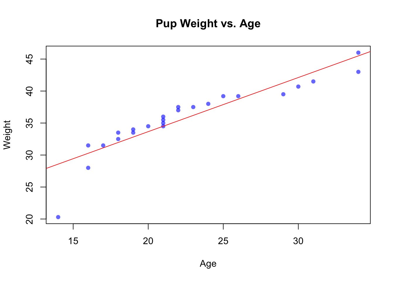

3.3.2 Reverse Regression

You can try reversing the roles of weight and age and repeating the above steps to see what results you get. Specifically, weight is now \(X\) instead of \(Y\), and age is now \(Y\) instead of \(X\). This is called reverse regression.

revreg <- lm(age ~ weight)

plot(age ~ weight,
     main = "Pup Age vs. Weight", xlab = "Weight", ylab = "Age",
     pch = 16, col = rgb(0,0,1,0.6))
abline(revreg, col = "red")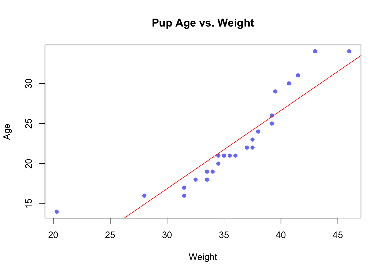

If we wish to plot both kinds of regression line on the same plot, we need to do a little bit of algebra. If we have two lines \(Y = a_y + b_y X\) and \(X = a_x + b_x Y\), and we want to plot them both at the same time, we need to solve both equations for \(Y\). The first is already done, and the second solves to \[ Y = -\frac{a_x}{b_x} + \frac{1}{b_x} X. \]

If we want to do this with code, we need a couple of additional tools. We can get the regression coefficients from the output of lm() by accessing the coefficients variable inside it. Like so,

revreg$coefficients

## (Intercept)      weight 
## -12.3781729   0.9751875

ax <- revreg$coefficients[1]
bx <- revreg$coefficients[2]

We can calculate the reversed intercept and slope using the above formula.

axy = -ax / bx
bxy = 1 / bx

The second tool is that we can plot any line we like by supplying abline with an intercept and slope.

plot(weight ~ age,
     main = "Pup Weight vs. Age", xlab = "Age", ylab = "Weight",
     pch = 16, col = rgb(0,0,1,0.6))
abline(reg, col = "red")
abline(a = axy, b = bxy, col = "black")
legend("bottomright", legend = c("weight on age", "age on weight"),
       lty = 1, col = c("red", "black"))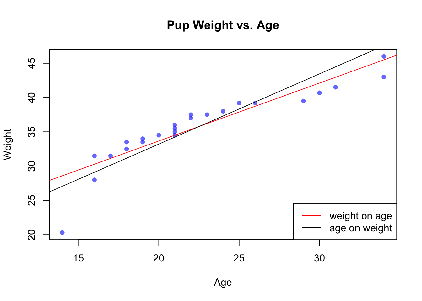

Notice that the lines are close, but not perfectly coincident. This is because minimizing the squared residuals of weight versus age results in a different line than minimizing the squared residuals of age versus weight.

Exercises

1. Make boxplots of:
   1. Age by ClutchID,
   2. Length by ClutchID
2. Think about why \(a_y\) and \(b_y\) are different for the regression of \(Y\) on \(X\) versus the (algebraicly reversed) \(a_{rev} = -\frac{a_x}{b_x}\) and \(b_{rev} = \frac{1}{b_x}\) for the reverse regression of \(X\) on \(Y\). When do you think they would be equal?