6.1 Confidence Intervals

It is simple to calculate confidence intervals in R. If we know the population standard deviation, we typically use the z.test() function from the BSDA package. We supply the population standard deviation and the confidence level like so,

library("BSDA")
z.test(choc, sigma.x = 2, conf.level = 0.95)$conf.int

## [1] 39.94773 40.02613
## attr(,"conf.level")
## [1] 0.95

If we do not know the population standard deviation, we typically use the t.test() function included in R by default. We supply the confidence level like so,

t.test(choc, conf.level = 0.95)$conf.int

## [1] 39.94724 40.02661
## attr(,"conf.level")
## [1] 0.95

6.1.1 Illustrating Confidence Intervals

The interpretation of confidence intervals can be summarised as follows: if repeated samples were taken and the 95% confidence interval computed for each sample, 95% of the intervals would contain the population mean. Let’s see if we can simulate what this statment implies through the example below.

Say we send a bunch of people to the chocolate factory to sample and measure the mean weight of the chocolate bars. They each take a sample of 20 bars, and construct a 95% confidence interval from their sample:

choc.batch <- rnorm(n = 20, mean = 40, sd = 2)
z.test(choc.batch, sigma.x = 2, conf.level = 0.95)$conf.int

## [1] 38.73064 40.48369
## attr(,"conf.level")
## [1] 0.95

Let’s tally how many of their confidence intervals covered the true mean. The following code simulates the process of repeatedly sampling batches of 20 bars, and constructing confidence intervals from each sample. One thousand batches are sampled in the code below. (Don’t worry about the large block of code, we will not expect you to plot things like this, but it is an illustration of what R is capable of.)

attempts = 1000
curve(expr = dnorm(x, mean = 40, sd = 2), from = 33, to = 48,
      main = "95% CI simulation results for sample size = 20",
      xlab = "Chocolate Bar Weight (in g)", ylab = "Density",
      lwd=2, col="blue")
abline(v = 40, col = "purple", lwd = 2)
failed_to_contain <- 0
for (i in 1:attempts) {
    col <- rgb(0,0,0,0.5)
    choc.batch <- rnorm(n = 20, mean = 40, sd = 2) 
    myCI <- z.test(choc.batch, sigma.x = 2, conf.level = 0.95)$conf.int
    if (min(myCI) > 40 | max(myCI) < 40) {
        failed_to_contain <- failed_to_contain + 1
        col <- rgb(1,0,0,1)
    }
    segments(min(myCI), 0.2 * i / attempts,
             max(myCI), 0.2 * i / attempts,
             lwd = 1, col = col)
}

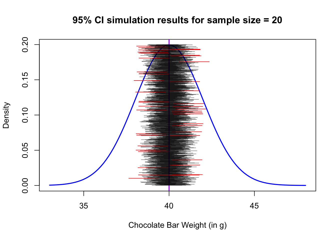
This illustrates nicely how the confidence intervals are correct a specified percentage of the time, and that percentage is the confidence level.

In this case, for a 95% CI, notice that approximately 5% of the confidence intervals we constructed actually DO miss the true mean (the ones in red).

failed_to_contain / attempts

## [1] 0.044