7.2 Checking Model Assumptions

The term “model diagnostics” refers to a range of plots and statistical tests that are used to evaluate both the assumptions and fit of a linear model. In R, there is an easy way to generate the most commonly used residual diagnostic plots:

par(mfrow=c(2,2))
plot(lin.model, pch = 16, col = rgb(0, 0, 0, 0.5))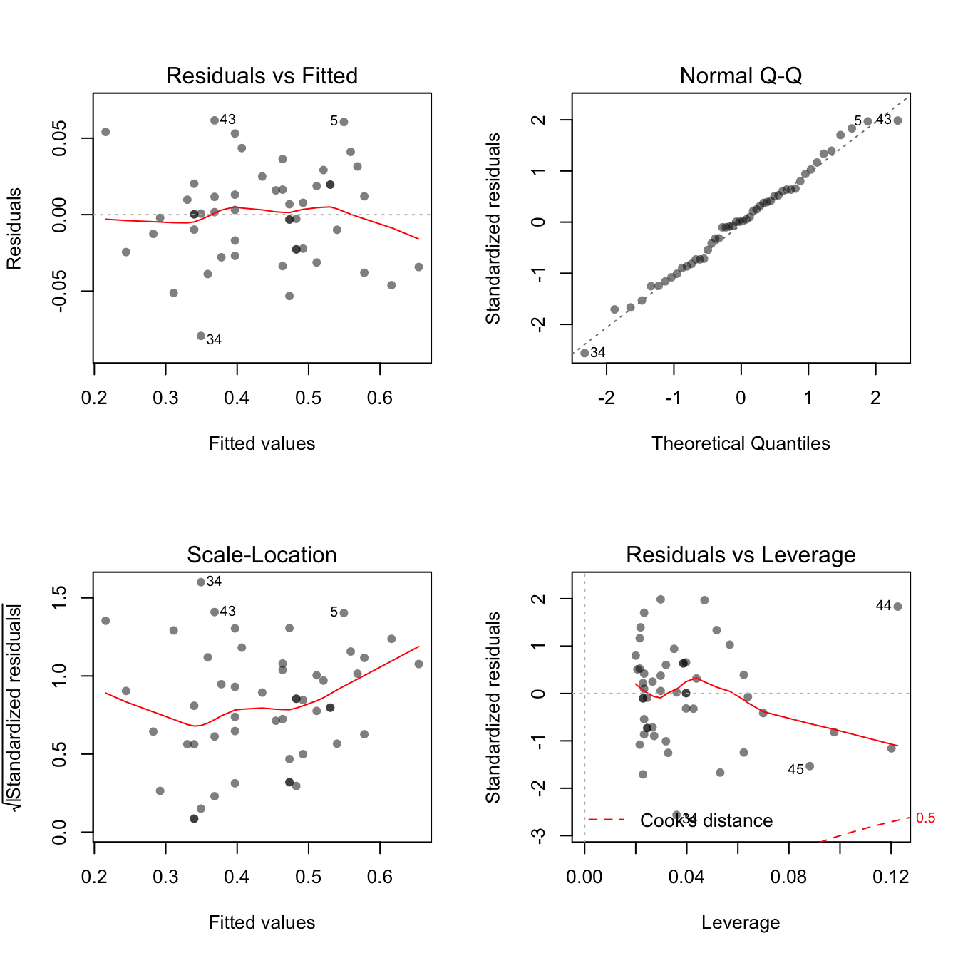

The four plots here provide a lot of information. We will focus on the the first two. To make sure we understand these, we are going to build them up directly using the elements of the lin.model object.

The assumptions for linearity and homoscedasticity (variance does not depend on Y) can be checked by plotting the residuals vs fitted. A “good” residual plot should have no noticeable patterns.

plot(lin.model$residuals ~ lin.model$fitted.values,
     main = "Residual plot", xlab = "Fitted Value", ylab = "Residual",
     pch = 16, col = rgb(0, 0, 0, 0.5))
abline(h = 0, col = "red")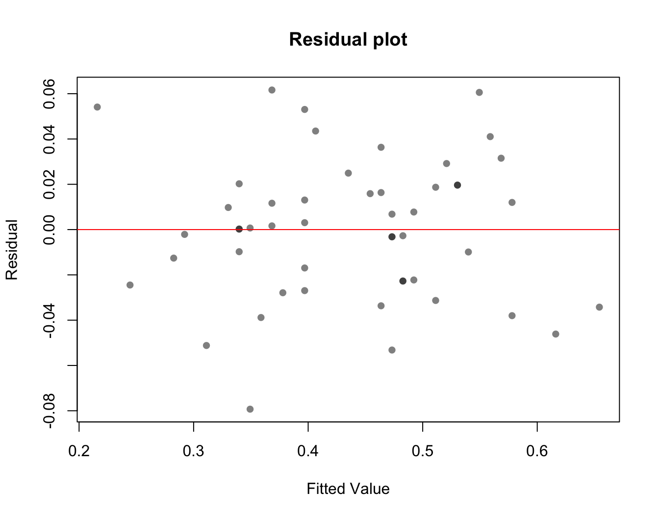

One of the other main assumptions we can check is whether the residuals are Normally distributed. The statistical tests we are using assume that: \(\epsilon_i \sim Normal(0, \sigma^2)\).

You can quickly check the normality assumption with a QQ-plot of the residuals. Remember that the QQ-plot compares the quantiles of the observed data (our residuals) to the quantiles of the standard normal.

qqnorm(lin.model$residuals,
       xlab = "Standard normal", ylab = "Residuals",
       pch = 16, col = rgb(0, 0, 0, 0.5))
qqline(lin.model$residuals, col = "red")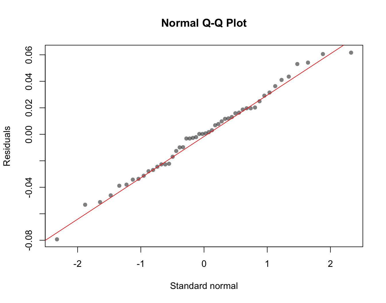

The pattern in the QQ-plot looks pretty good. This suggests the residuals are approximately normally distributed, and this assumption needed for our statistical tests is met.