9.7 Regression Inference
Learning Objectives
Useful Functions
Dataset: State-level Presidential Election Data
We saw in the tutorial that the relationship between the statewide Democratic voting fraction in 2012 and 2016 was very strong. Now, let’s take a look at the data from 2004 (Bush vs Kerry) and see how it compares to the election last November.
If you did not save the data from Tuesday section, read it in again using these commands.
election_all <- readr::read_csv("election04-16.csv")
DC <- subset(election_all, State == "Washington DC")
election <- subset(election_all, State != "Washington DC")
The scatterplot for 2016 vs. 2004 is shown below. Note that we identify the DC data on the plot, but we are excluding it when we fit the linear model (lm(Y2016 ~ Y2004, data=election) where the election dataframe excludes DC)
plot(Y2016 ~ Y2004, data=election, xlim=c(0.25, 0.95), ylim=c(0.25, 0.95),
     main="Proportion of Votes for Democratic Candidate", xlab="2004", ylab="2016",
     pch = 16, col = rgb(0, 0, 0, 0.5))

points(Y2016 ~ Y2004, data=DC, pch = 16, col = rgb(0, 0, 1, 1))
text(Y2016 ~ Y2004, data=DC,
     label='DC', col='blue', pos=2, cex=0.8)

abline(lm(Y2016 ~ Y2004, data=election), col='red')
abline(0,1, col="gray", lty=2)
legend("topleft", legend=c("y=x", "Regression Line (DC excl)"),
       lty=c(2,1), col=c("gray","red"))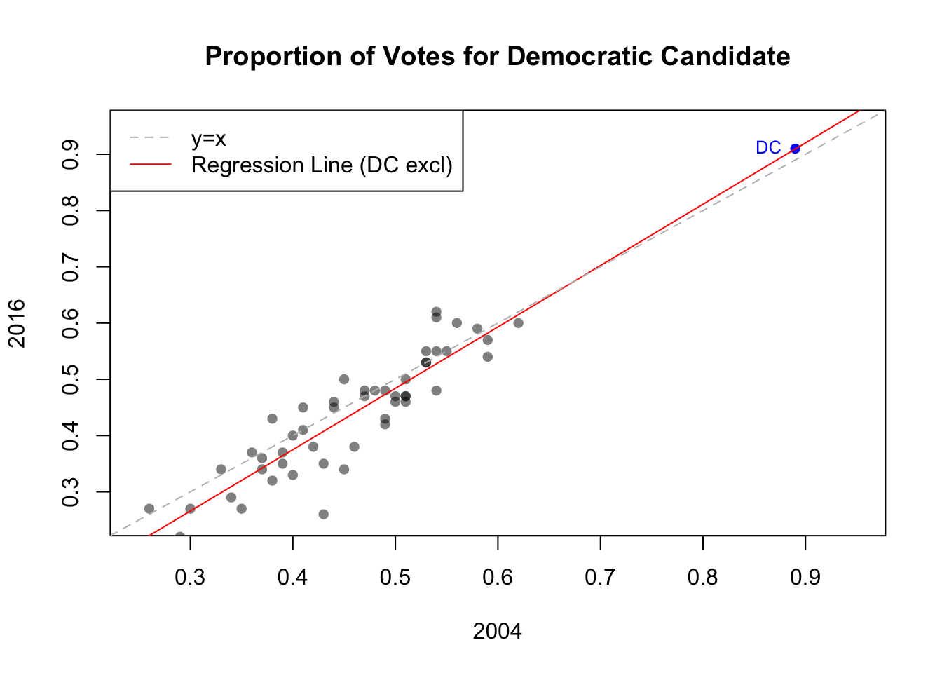
Fit a linear regression model to these data, excluding DC, using 2004 as the predictor and 2016 as the response. Use the output to answer the following questions.
9.7.1 Testing Coefficients
What is the value of the t-statistic for the
Y2004variable?What is the p-value of the t-test for the significance of the
Y2004variable?Is there significant association, as measured by the regression slope coefficient, between the 2004 and 2016 election results?
What proportion of the variation in
Y2016is explained by the predictorY2004?Look at the DC data (the code for extracting this is in the tutorial). Take the proportion Democratic vote in 2004 and use it to constuct the prediction interval for DC in 2016. What is the lower bound?.
What is the upper bound?
Is the observed Democratic vote proportion for DC in 2016 inside the prediction interval?
Further thoughts
Think about the DC datapoint. Does it have leverage? Influence? How does the prediction interval information help you think about the answer this question? Do you think DC would lie in the confidence interval for \(\mu_y | x\). Why or why not? Do you think the regression coefficient would change much if you included the DC datapoint? Keep this in mind as you work with the next dataset.
Dataset: Florida County-level Presidential Election Data
Unfortunately, voting discrepancies don’t just happen in corrupt governments. In the 2000 US Presidential election with George Bush vs Al Gore, the entire election was decided by the state of Florida which itself was decided by less than 600 votes (a margin of .009%). In particular, Palm Beach county used a butterfly ballot which was widely criticized for its confusing design (http://en.wikipedia.org/wiki/File:Butterfly_large.jpg). Many speculated that this may have caused a large number of voters who intended to vote for Al Gore to vote for Pat Buchanan (Reform Party) instead.
We would expect that the number of registered voters in 2000 who belonged to the Reform party should be a pretty good predictor of how many people ended up voting for Pat Buchanan.
We have combined county vote data (slightly altered) from Wikipedia with data from the Florida Division of Elections on the party affiliation of the registered voters in 2000. The predictor is the number of registered Reform voters (Reg.Reform). The response is the number who voted for Buchanan (Buch.Votes).
Run the following code to read in the data, fit the linear model, and produce a scatterplot of the results with the regression line:
florida = read.csv("FL.csv")
head(florida)
## County Reg.Dem Reg.Rep Reg.Reform Total.Reg Buch.Votes
## 1 Alachua 64,135 34,319 102 120,867 284
## 2 Baker 10,261 1,684 13 12,352 99
## 3 Bay 44,209 34,286 64 92,749 291
## 4 Bradford 9,639 2,832 11 13,547 65
## 5 Brevard 107,840 131,427 156 283,680 598
## 6 Broward 456,789 266,829 339 887,764 823palm = subset(florida, County=="Palm") # extract Palm County
lin.mod = lm(Buch.Votes ~ Reg.Reform, data=florida)
plot(Buch.Votes ~ Reg.Reform, data=florida,
main = "Registered Voters vs Actual Votes",
xlab = "Registered Reform Voters", ylab = "Actual Votes",
pch = 16, col = rgb(0, 0, 0, 0.5))
# Identify Palm County on the plot
text(Buch.Votes ~ Reg.Reform, data=palm,
label='Palm', pos=2, col="blue")
abline(lin.mod, col = "red")
9.7.2 Checking for an Outlier
Does Palm County appear to be an outlier?
Does Palm County appear to be an influential point?
What proportion of the variation in Buchanan votes is explained by the number of registered Reform voters in this model?
Use the code below to remove Palm county, and fit another model to the new data. We will use the prediction interval to assess whether Palm County is an outlier.
florida.NoPalm = florida[-which(florida$County=="Palm"),]
lin.mod.NoPalm = lm(Buch.Votes ~ Reg.Reform, data=florida.NoPalm) plot(Buch.Votes ~ Reg.Reform, data=florida,
main = "Registered Voters vs Actual Votes",
xlab = "Registered Reform Voters", ylab = "Actual Votes",
pch = 16, col = rgb(0, 0, 0, 0.5))
text(Buch.Votes ~ Reg.Reform, data=palm,
label='Palm', pos=2, col="blue")
abline(lin.mod, col = "red")
abline(lin.mod.NoPalm, col = "blue")
legend("topleft",
legend=c("regression with Palm data",
"regression without Palm data"),
lwd=1, col=c('red','blue'))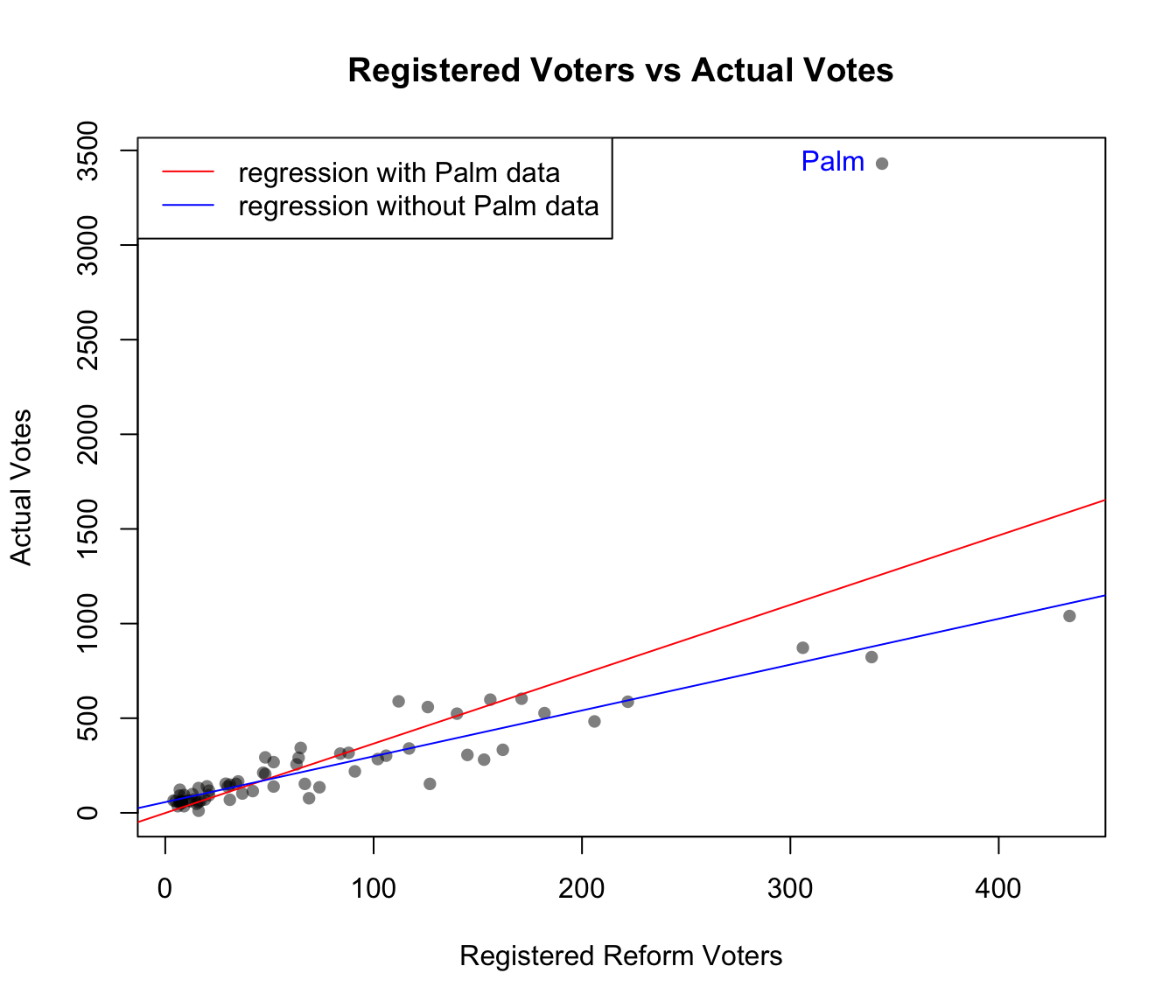
From the new model with Palm County excluded, lin.mod.NoPalm, answer the following questions:
What is the new estimate for the \(\beta_1\) coefficient (slope associated with
Reg.Reform)?What is the value of the t-statistic for the
Reg.Reformvariable?What is the p-value of the t-test for the significance of the
Reg.Reformvariable?Is there significant association between registered Reform voters and votes for Buchanan?
What proportion of the variation in votes for Buchanan is now explained by the number of registered Reform Party voters?
Does the exclusion of Palm County lead to a better model fit?
Use regression diagnostics to check the assumptions needed for valid statistical inference for this linear model. Do these suggest the assumptions for valid inference are met?
- No, because we see systematic nonlinearity
- No, because we see heteroscedasticity and a right skewed distribution
- No, because we see nonzero regression coefficients
- Yes, all assumptions are valid for this data
Now try a log-transformation using this code:
logmod <- lm(log1p(Buch.Votes) ~ log1p(Reg.Reform), data=florida.NoPalm)

plot(log1p(Buch.Votes)~log1p(Reg.Reform), data=florida.NoPalm,
     main='Regression, log scale', xlab='log Reg.Reform', ylab='log Buch.Votes',
     pch = 16, col = rgb(0, 0, 0, 0.5))
abline(logmod, col='red')
plot(logmod$residual ~ log1p(florida.NoPalm$Reg.Reform),
     main="Residual plot", xlab="Reg.Reform", ylab="Residuals",
     pch = 16, col = rgb(0, 0, 0, 0.5))
abline(h=0, col='red')
Compare the new scatter plot after the log transformations to the original unlogged version. What do you see?
- The log-transformation introduced systematic nonlinearity
- The log-transformation eliminated the right skew from both variables
- The log-transformation reduced all regression coefficients to zero
- The log-transformation had no noticeable effect
Compare the new residual plot after the log transformations to the original unlogged residual plot.
- The log-transformation made the skew worse
- The log-transformation caused the residuals to have a nonzero mean
- The log-transformation eliminated the heteroscedasticity from the residuals
- The log-transformation had no noticeable effect
Let’s take a closer look at the data for Palm county:
print(palm)## County Reg.Dem Reg.Rep Reg.Reform Total.Reg Buch.Votes
## 50 Palm 295,185 231,233 344 656,694 3430The number of registered Reform voters in Palm was 344 and the number of Buchanan voters in Palm was 3430
Using
lin.mod.NoPalm, what is the predicted number of votes for Buchanan in Palm County?What is the lower bound of the 95% prediction interval for Palm County?
What is the upper bound of the 95% prediction interval for Palm County?
Is the observed value for
Buch.Votesin Palm County inside this prediction interval?What is the prediction error? (Note this is similar to residual, but not a residual because we did not use Palm County to fit our model)