9.5 Distributions and the CLT
Learning Objectives
- Learn to work with distribution functions.
- Learn how the Central Limit Theorem (CLT) shows up in data.
Useful Functions
- Use
dpois()to calculate the PDF of the Poisson distribution. Use
ppois()to calculate the CDF of the Poisson distribution.Use
qqnorm()andqqline()to visually assess the normality of a sample.
9.5.1 The Poisson distribution
Assume that the number of calls to the U-District fire station in a week, \(X\), follows a Poisson distribution with \(\lambda = 14\). The Poisson distribution is a discrete distribution with the probability mass function: \[p(x) = \frac{e^{-\lambda} \lambda^x}{x!}, ~ x=0,1,2,\ldots\]
The mean and variance of a Poisson distributed random variable parameterized by \(\lambda\) are both \(\lambda\). This means that the average number of calls received by the fire station in a given week is 14.
First, let’s look at how different a Poisson(14) is from the Normal distribution.
set.seed(76192)
dat <- rpois(1000, lambda = 14)
qqnorm(dat, pch = 16, col = rgb(0, 0, 0, 0.5))
qqline(dat, col = rgb(1, 0, 0, 0.6))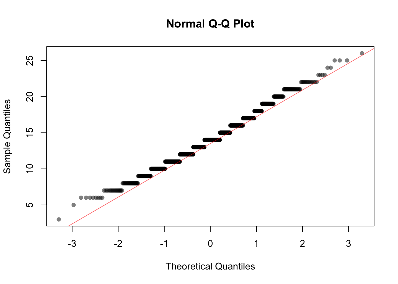
You can clearly see the discrete values of the Poisson in this plot, but apart from this what does the plot suggest about the similarity/difference between these two distributions?
Now let’s see how the sampling distribution of the mean from a Poisson behaves.
For this lab, we simulate 1000 samples (replicates) from \(X\) of sizes \(n = 5, 20\), and \(50\) and calculate the sample mean each time (which we refer to as \(\overline{X}_5, \overline{X}_{20}\) and \(\overline{X}_{50}\) respectively).
Use the following code to generate the samples:
set.seed(199001)
x5bar <- replicate(1000, mean(rpois(5, lambda = 14)))
x20bar <- replicate(1000, mean(rpois(20, lambda = 14)))
x50bar <- replicate(1000, mean(rpois(50, lambda = 14)))
We use the following code to plot the histogram and the QQ-plot of each of the sampling distributions:
par(mfrow=c(1,2))
hist(x5bar, breaks=20, xlim=c(0.5 * 14, 1.5 * 14), freq = FALSE)
qqnorm(x5bar, ylab="x5bar", pch = 16, col = rgb(0, 0, 0, 0.5))
qqline(x5bar, col = rgb(1, 0, 0, 0.6))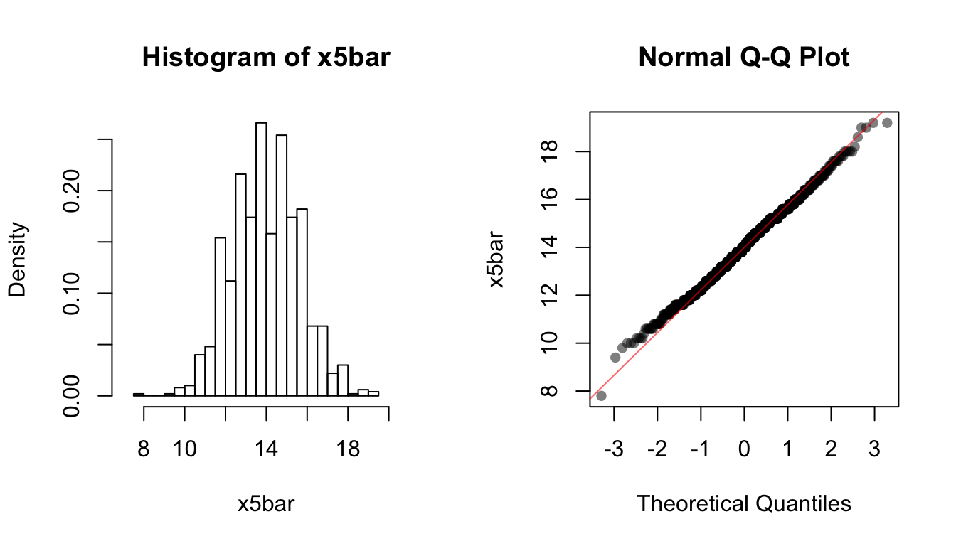
hist(x20bar, breaks=20, xlim=c(0.5 * 14, 1.5 * 14), freq = FALSE)
qqnorm(x20bar, ylab="x20bar", pch = 16, col = rgb(0, 0, 0, 0.5))
qqline(x20bar, col = rgb(1, 0, 0, 0.6))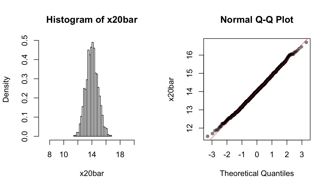
hist(x50bar, breaks=20, xlim=c(0.5 * 14, 1.5 * 14), freq = FALSE)
qqnorm(x50bar, ylab="x50bar", pch = 16, col = rgb(0, 0, 0, 0.5))
qqline(x50bar, col = rgb(1, 0, 0, 0.6))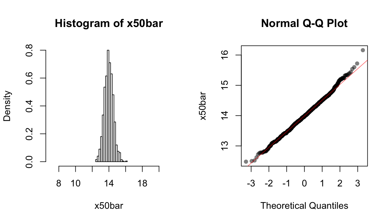
Questions
For this scenario, round to TWO decimal places.
What is the theoretical expectation for \(\overline{X}_5\)?
Are the theoretical expectations for \(\overline{X}_5\), \(\overline{X}_{20}\) and \(\overline{X}_{50}\) all the same?
Use R to calculate the means of the sampling distributions you simulated above (x5bar, x20bar, and x50bar).
What is the sample mean of the simulated
x5bar?What is the sample mean of the simulated
x20bar.What is the sample mean of the simulated
x50bar.Using the PDF, calculate the probability that the fire station will receive exactly 10 calls in a week.
Using the CDF, calculate the probability that the fire station will receive less than or equal to 11 calls in a week.
9.5.2 The Exponential distribution
If the number of calls per week follows a Poisson distribution with mean \(\lambda\), the wait times between calls \(Y\) follows an Exponential distribution with mean \(1/\lambda\) (or equivalently, rate \(\lambda\)), and variance \(1/\lambda^{2}\).
As before, let’s first look at how different an Exponential(1/14) is from the Normal distribution.
dat <- rexp(1000, rate = 14)
qqnorm(dat, pch = 16, col = rgb(0, 0, 0, 0.5))
qqline(dat, col = rgb(1, 0, 0, 0.6))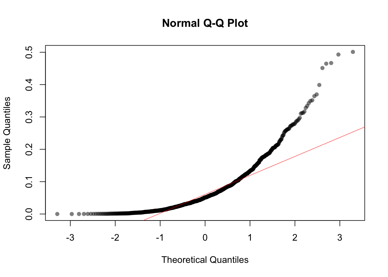
What does the plot suggest about the similarity/difference between the Normal and the Exponential(1/14) distributions? Is it the same or different than the comparison between the Normal and the Poisson(14)?
Now let’s see how the sampling distribution of the mean from an Exponential behaves.
Repeat the simulation study above, this time for \(Y\).
Use the following code to generate the samples:
set.seed(81793)
y5bar <- replicate(1000, mean(rexp(5, rate = 14)))
y20bar <- replicate(1000, mean(rexp(20, rate = 14)))
y50bar <- replicate(1000, mean(rexp(50, rate = 14)))
We use the following code to plot the histogram and the QQ-plot of each of the sampling distributions:
par(mfrow=c(1,2))
hist(y5bar, breaks = 20, xlim = c(0, 4/14), freq = FALSE)
qqnorm(y5bar, ylab = "y5bar", pch = 16, col = rgb(0, 0, 0, 0.5))
qqline(y5bar, col = rgb(1, 0, 0, 0.6))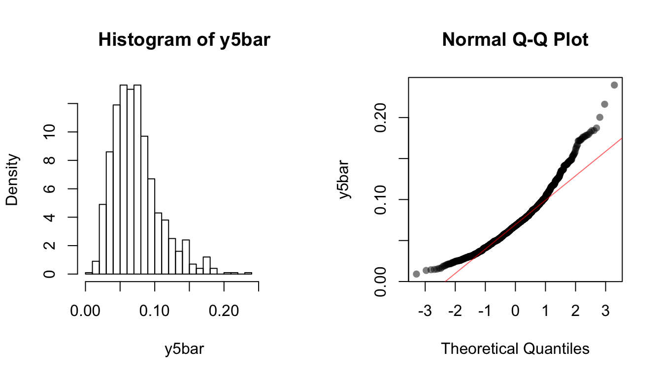
hist(y20bar, breaks = 20, xlim = c(0, 4/14), freq = FALSE)
qqnorm(y20bar, ylab = "y20bar", pch = 16, col = rgb(0, 0, 0, 0.5))
qqline(y20bar, col = rgb(1, 0, 0, 0.6))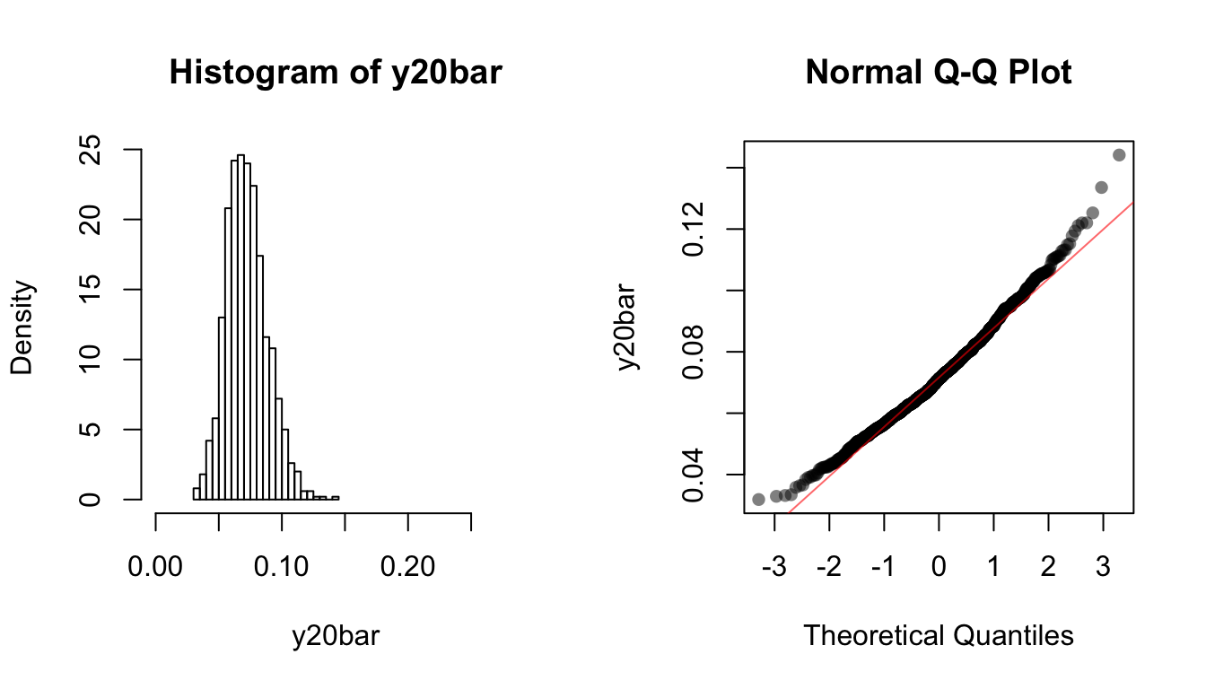
hist(y50bar, breaks = 20, xlim = c(0, 4/14), freq = FALSE)
qqnorm(y50bar, ylab = "y50bar", pch = 16, col = rgb(0, 0, 0, 0.5))
qqline(y50bar, col = rgb(1, 0, 0, 0.6))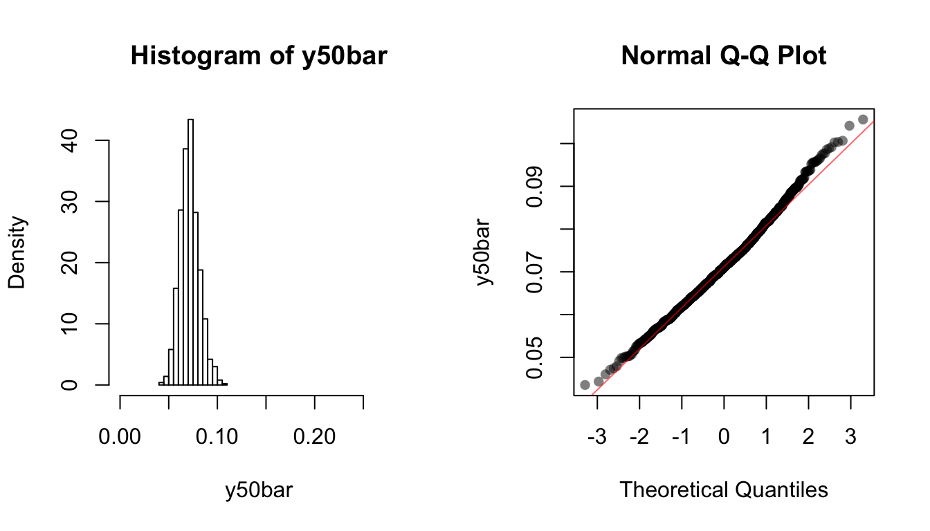
Note how the skewness goes away as sample size gets larger.
Questions
For this scenario, round to THREE decimal places
What is the theoretical expectation for \(\overline{Y}_5\)?
Are the theoretical expectations for \(\overline{Y}_5\), \(\overline{Y}_{20}\) and \(\overline{Y}_{50}\) all the same?
Use R to calculate the means of the sampling distributions you simulated above (y5bar, y20bar, and y50bar).
What is the sample mean of the simulated
y5bar?What is the sample mean of the simulated
y20bar?What is the sample mean of the simulated
y50bar?
9.5.3 The CLT, sample size, and asymptotic normality
What does Central Limit Theorem (CLT) actually tell us about distributions of random variables?
- The CLT says that, with a large enough sample, an Exponentially distributed random variable will approximate a Normal distribution.
- The CLT says that all of the sample statistics from an Exponentially distributed random variable will have a distribution that approaches Normality as the number of replications used for the sampling distribution increases.
- The CLT says that the sample mean of an Exponentially distributed random variable will approach the mean of a Poisson distributed random variable, as the sample size increases.
- The CLT says that the sample means for most (but not all) distributions will have a distribution that approaches Normality as the number of observations in the sample size used to calculate the mean gets larger.
- The CLT says that, with a large enough sample, an Exponentially distributed random variable will approximate a Normal distribution.
What do you observe about the impact of sample size on the expected value of the sample mean?
- There is no clear impact of sample size on the expected value.
- Smaller sample sizes lead to expected values that underestimate the mean.
- Larger sample sizes lead to expected values that overestimate the mean.
- None of these.
What do you observe about the impact of sample size on the approximate normality of the sampling distribution for the mean of the Poisson(14) RV?
- As sample size increases, approximate normality is obtained quickly (sample size of 50 is sufficient).
- As sample size increases, approximate normality is obtained slowly (requires sample size greater than 50).
- Approximate normality will never be attained at any sample size.
- None of these.
What do you observe about the impact of sample size on the approximate normality of the sampling distribution for the mean of the Exponential(1/14) RV?
- As sample size increases, approximate normality is obtained faster than for Poisson(14).
- As sample size increases, approximate normality is obtained slower than for Poisson(14).
- Approximate normality will never be attained at any sample size.
- None of these.
- As sample size increases, approximate normality is obtained faster than for Poisson(14).
What does this suggest about using the CLT in practice?
- The more symmetric the original distribution, the more quickly the sampling distribution of the mean will converge to a Normal distribution.
- The CLT does not apply to the sampling distribution of the mean of an Exponential distribution, because it is right skewed.
- The CLT does not apply to the sampling distribution of the mean of a Poisson distribution, because it is discrete.
- None of these.