5.3 Continuous Distributions
Continuous distributions are not restricted to being whole numbers and (depending on the distribution) can take decimal values like 1.54289 and -0.017982. As above, we will not (yet) go into why the distributions are the way they are, only what they look like, and how to sample data from them.
For each distribution, there are four functions that provide important capabilities.
The random sample function, with
rin the function name, generates (pseudo)random samples from the specified distribution.The density function, with
din the function name, calculates the probability (density) of a particular outcome. It is also known as the probability density function or PDF.The probability distribution function, with
pin the function name, calculates the probability of a range of outcomes. It is also known as the cumulative distribution function or CDF.The quantile function, with
qin the function name, calculates the range of outcomes required to add up to a particular probability. It is also known as the inverse CDF.
5.3.1 The Normal Distribution
There is a very important distribution in statistics called the Normal distribution. It is a bell-shaped distribution, and it shows up everywhere in nature and probability. It looks like this,
curve(dnorm(x), xlim = c(-3, 3),
      main = "The Standard Normal Distribution", ylab = "Density")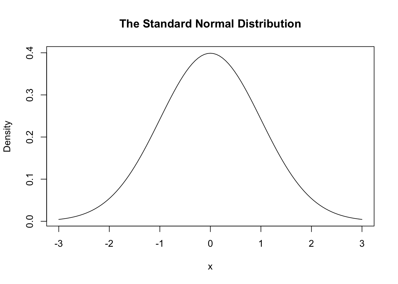
This bell-shape always stays the same, and it is sometimes called the Normal curve. However, there are two parameters that decide where the curve is centered and how wide and short versus thin and tall the curve is. The mean parameter (or \(\mu\)) specifies the center of the distribution, and the sd parameter (or \(\sigma\)) controls how wide the curve is.
curve(dnorm(x, mean = 2, sd = 0.5), xlim = c(-4, 4), col = "red",
      main = "The Normal Distribution", ylab = "Density")
curve(dnorm(x, mean = -1, sd = 1), xlim = c(-4, 4), add = TRUE, col = "blue")
text(x = c(-1, 2), y = c(0.2, 0.4), labels = c("N(-1, 1.0)", "N(2, 0.5)"),
     col = c("blue", "red"))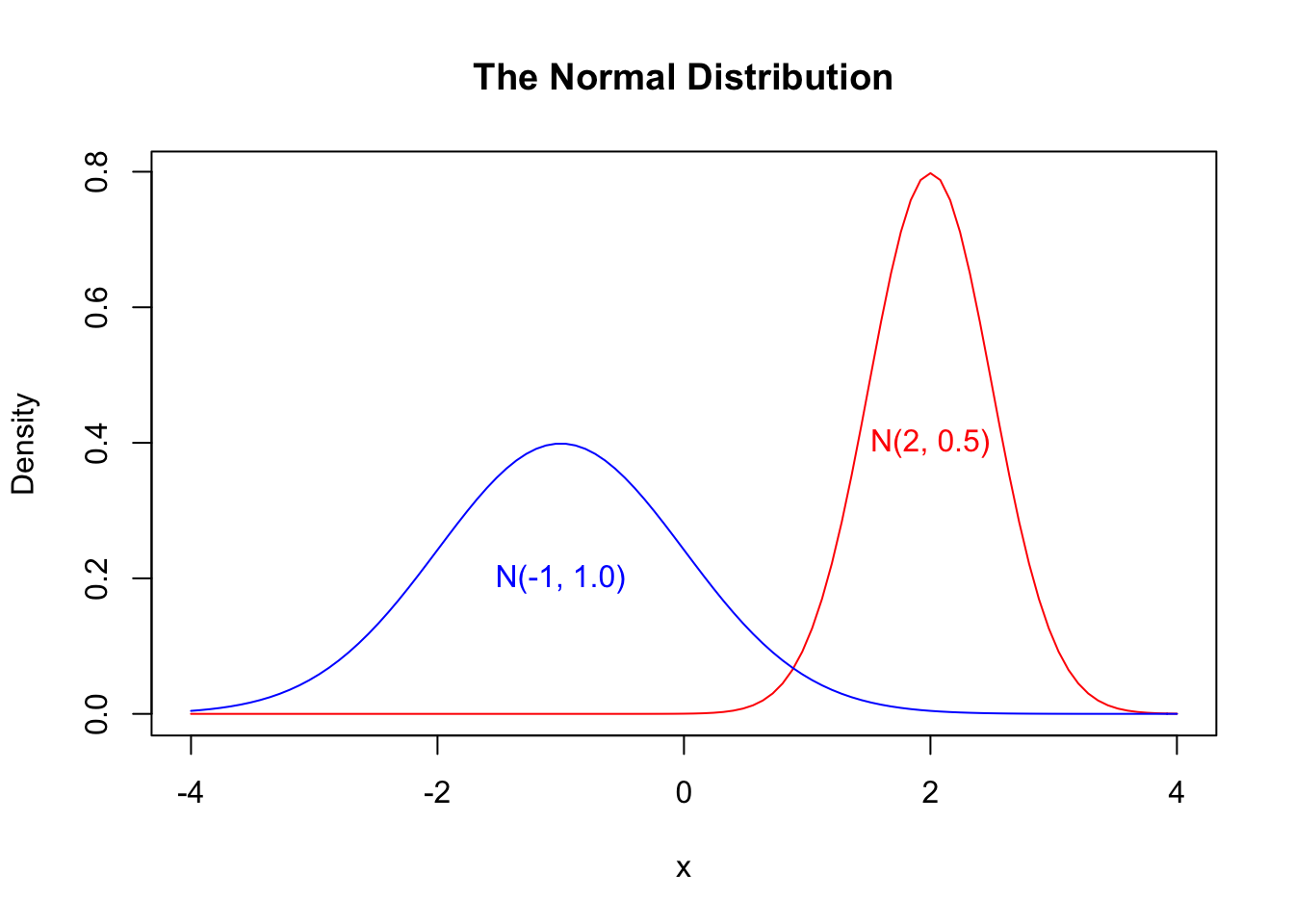
There is a special Normal distribution called the standard Normal which is simply a Normal distribution with mean 0 and standard deviation 1, as illustrated above (in the first figure of this section).
The (Standard) Normal CDF looks like this,
curve(pnorm(x), xlim = c(-3, 3),
      main = "The Standard Normal CDF", ylab = "Probability")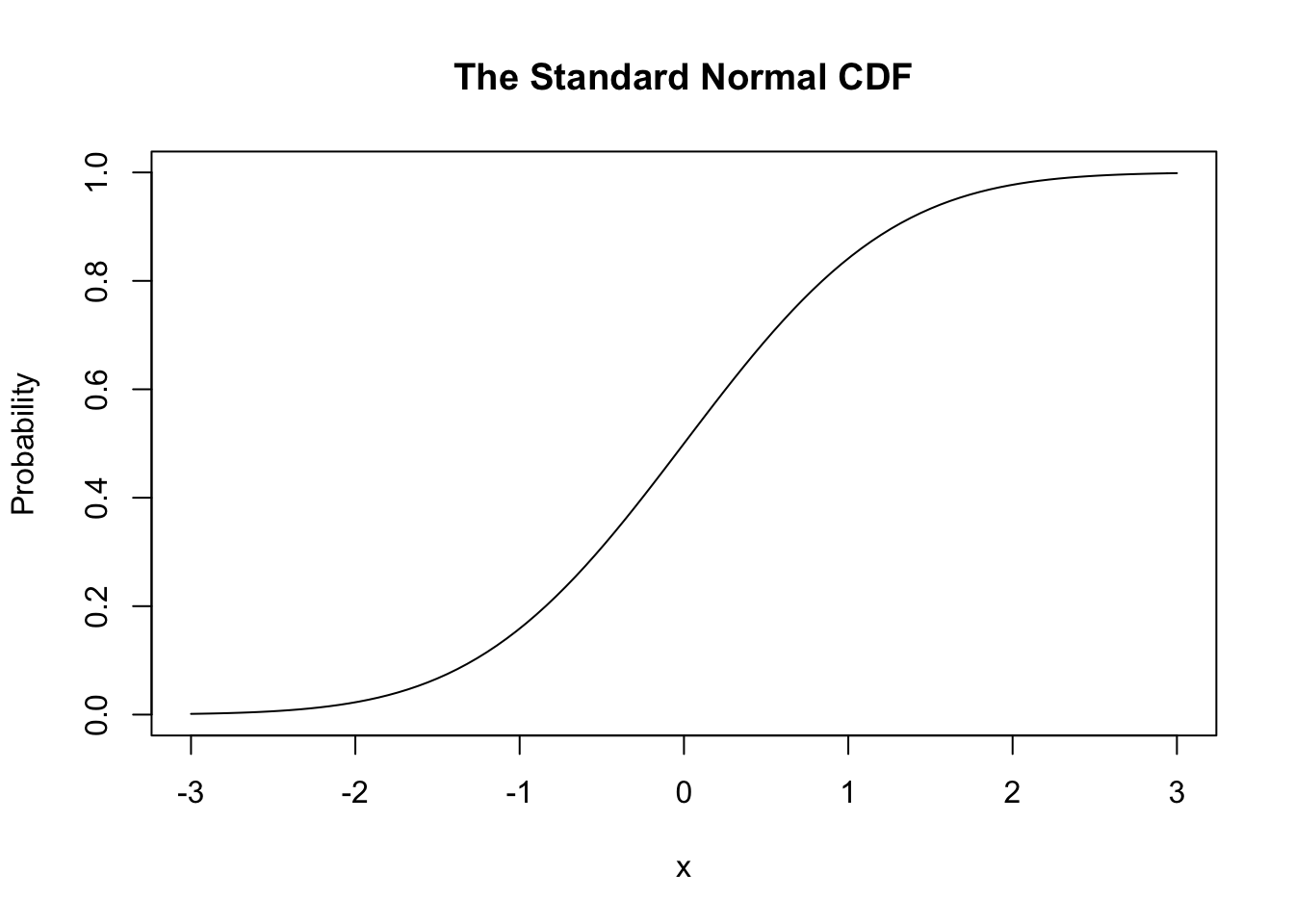
Sampling
We can sample from the Normal distribution with the rnorm() function.
rnorm(n = 5, mean = 5, sd = 2)## [1] 4.564656 7.496730 6.937214 5.514461 5.985538We can sample from the standard Normal very easily because mean = 0 and sd = 1 are the function’s default values.
rnorm(n = 5)## [1] 2.2130967 1.7633171 0.2901826 -1.3893091 2.1754976Plotting
The Normal is a continuous distribution, so we cannot use a standard bar plot. However, a histogram will be suitable.
samp <- rnorm(1000)
hist(samp, freq = FALSE, main = "Histogram of Normal data")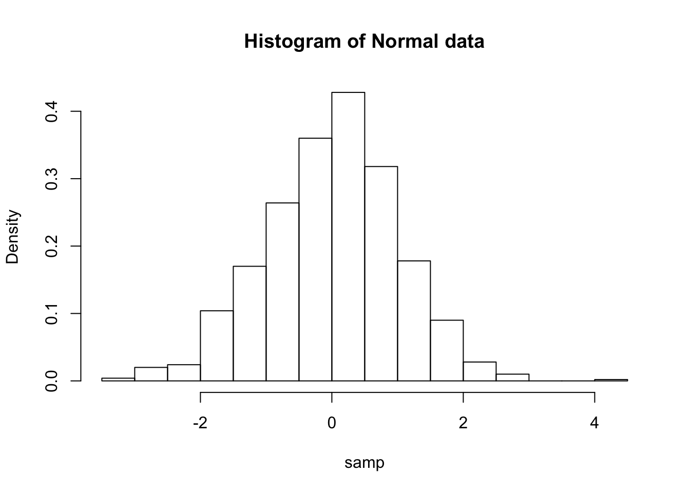
We can also plot an approximation to the continuous distribution based on our sample.
plot(density(samp), xlab = "x", ylab = "Density",
     main = "Approximate Distribution")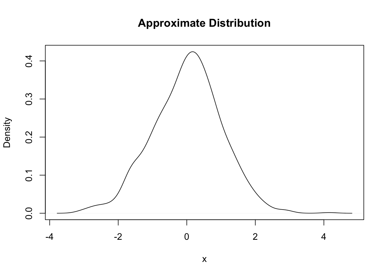
We can also check whether our data looks Normal using a Q-Q plot.
qqnorm(samp, pch = 16, col = rgb(0, 0, 0, 0.5))
qqline(samp, col = "red")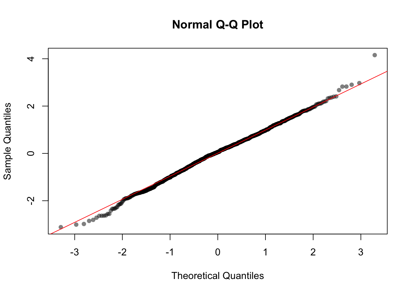
Here our data closely follows the ideal line, which confirms that our data is Normal.
5.3.2 The Uniform Distribution
One common distribution is called the uniform distribution. It represents the distribution where every value between min and max is equally likely.
We can sample from the uniform distribution using the runif() function. It takes three arguments:
n: how many data points we want to samplemin: the smallest possible value (default = 0)max: the largest possible value (default = 1)
runif(n = 5, min = -1, max = 2)## [1] 1.1182651 -0.6040557 -0.1208399 -0.9949078 0.2459637As above, since the uniform distribution is continuous, we use a histogram to see the shape of the data. We sample 10000 data points from this min = -1, max = 2 uniform distribution:
data = runif(n = 10000, min = -1, max = 2)
hist(data, xlim = c(-2, 3), main = "Histogram of Unif(min = -1, max = 2)")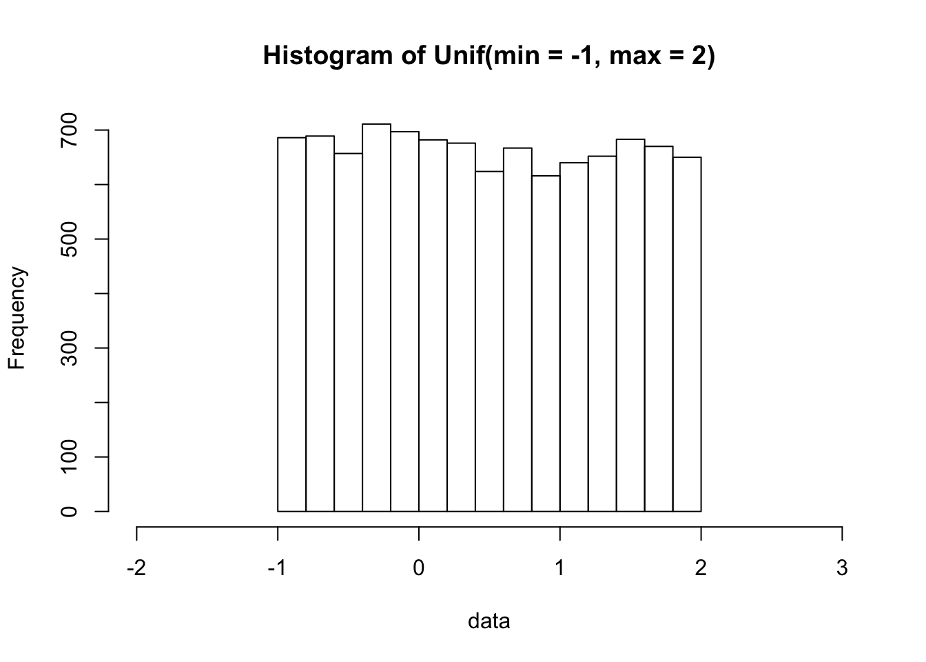
Its PDF is very simple:
curve(dunif(x, min = -1, max = 2), xlim = c(-2, 3),
      main = "PDF of Unif(min = -1, max = 2)", ylab = "Density")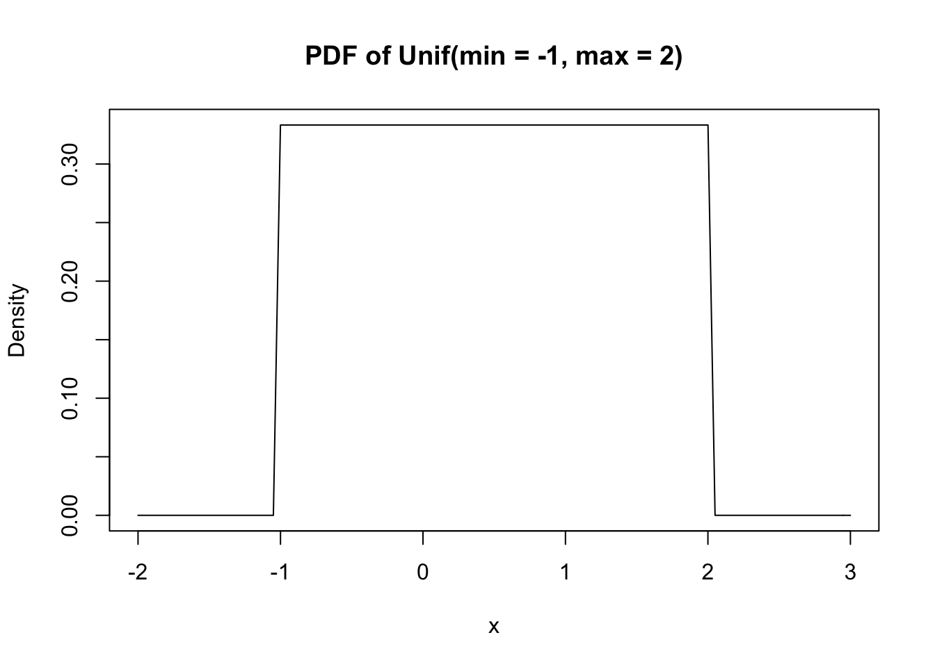
Its CDF is almost as simple:
curve(punif(x, min = -1, max = 2), xlim = c(-2, 3),
      main = "CDF of Unif(min = -1, max = 2)", ylab = "Probability")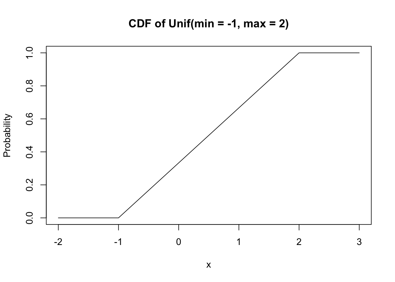
5.3.3 The Exponential Distribution
Another very common continuous distribution is called the Exponential distribution. We can sample from the exponential distribution using the rexp() function. It takes two arguments:
n: how many data points we want to samplerate: the rate that “successes” occur
rexp(n = 5, rate = 0.2)## [1] 4.8657688 6.4025406 5.1987466 0.1623184 1.0237677As above, since the exponential distribution is continuous, we use a histogram to see the shape of the data. We sample 10000 data points from this rate = 0.2 exponential distribution:
data = rexp(n = 10000, rate = 0.2)
hist(data, main = "Histogram of Exp(rate = 0.2)")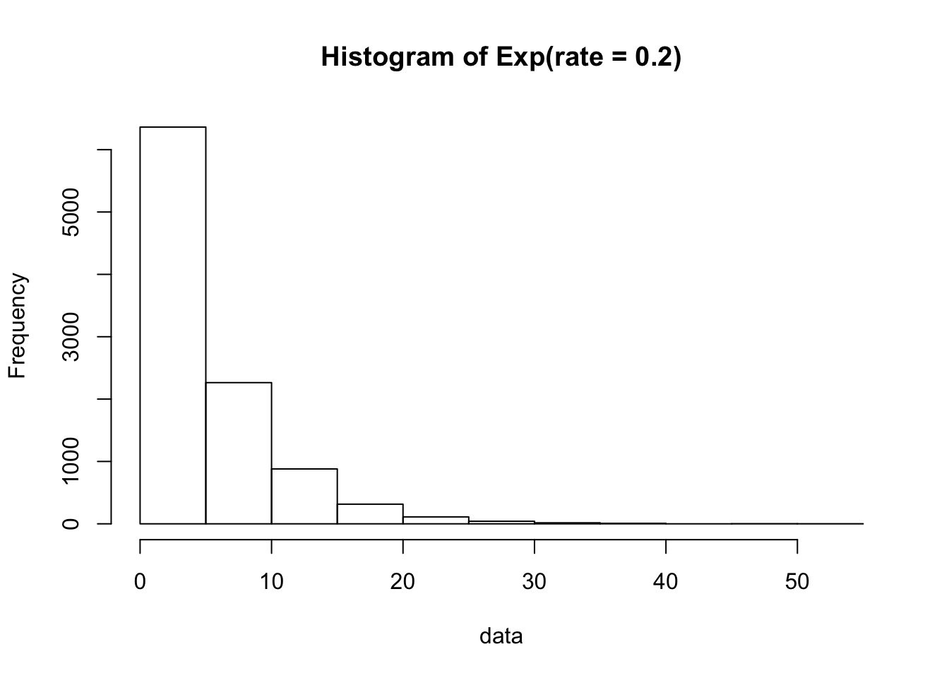
Its PDF is shown here:
curve(dexp(x, rate = 0.2), xlim = c(0, 50),
      main = "PDF of Exp(rate = 0.2)", ylab = "Density")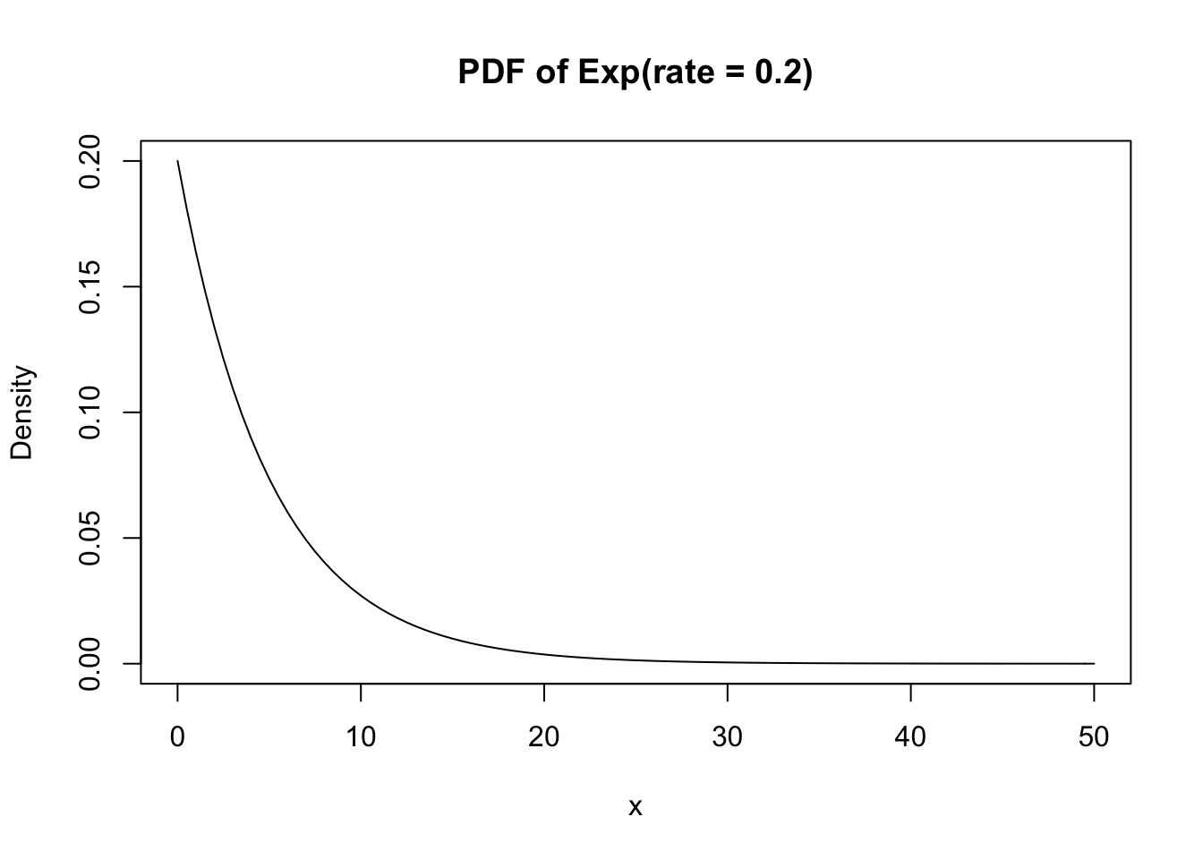
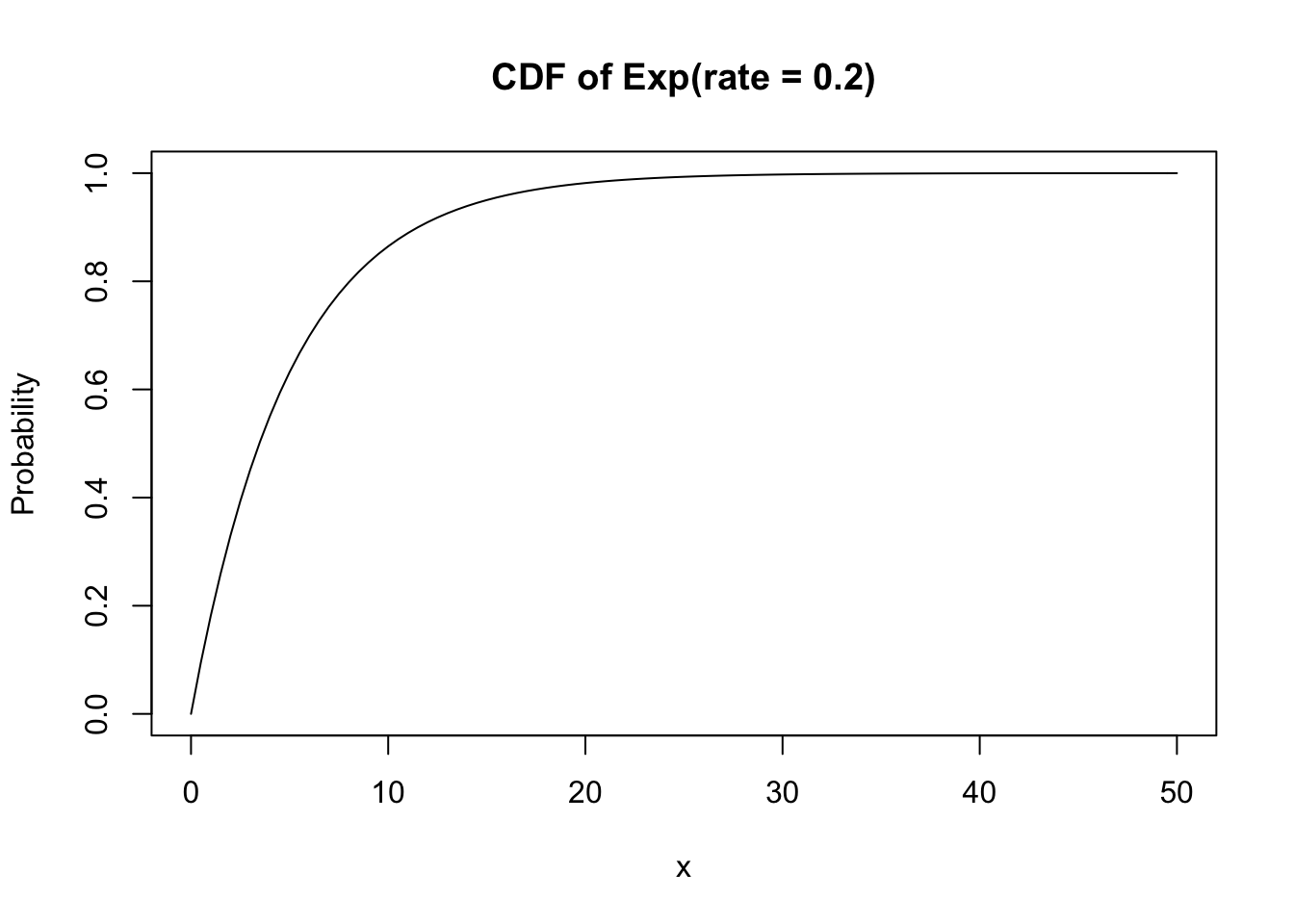
Its CDF is shown here:
curve(pexp(x, rate = 0.2), xlim = c(0, 50),
      main = "CDF of Exp(rate = 0.2)", ylab = "Probability")