5.2 Discrete Distributions
Discrete random variables can only result in whole numbers (0, 1, 2, …). Here we explore a couple of the most common kinds of discrete distributions. We will not (yet) go into why the distributions are the way they are, only what they look like, and how to sample data from them.
For each distribution, there are four functions that provide important capabilities.
The random sample function, with
rin the function name, generates (pseudo)random samples from the specified distribution.The density function, with
din the function name, calculates the probability (density) of a particular outcome. It is also known as the probability density function or PDF.The probability distribution function, with
pin the function name, calculates the probability of a range of outcomes. It is also known as the cumulative distribution function or CDF.The quantile function, with
qin the function name, calculates the range of outcomes required to add up to a particular probability. It is also known as the inverse CDF.
5.2.1 The Bernoulli Distribution
A Bernoulli random variable (\(X \sim \text{Bernoulli}(p)\)) is equivalent to a (not necessarily fair) coin flip, but the result is just 0 or 1. The parameter \(p\) is the probability of getting a 1. The best way to simulate this is using the binomial distribution (more below), for which the Bernoulli is a special case (size = 1).
rbinom(1, size = 1, p = 0.7)## [1] 1We can also randomly draw a whole bunch of Bernoulli trials:
rbinom(20, size = 1, p = 0.7)## [1] 0 1 1 1 0 0 1 1 0 1 0 1 1 1 1 1 0 0 1 1Distribution Functions
The Bernoulli has a very simple PDF, with \(X = 1\) having probability \(p\) and \(X = 0\) having probability \(1-p\).
barplot(names.arg = 0:1, height = dbinom(0:1, size = 1, p = 0.7),
        main = "Bernoulli PDF", xlab = 'X', ylab = 'Probability')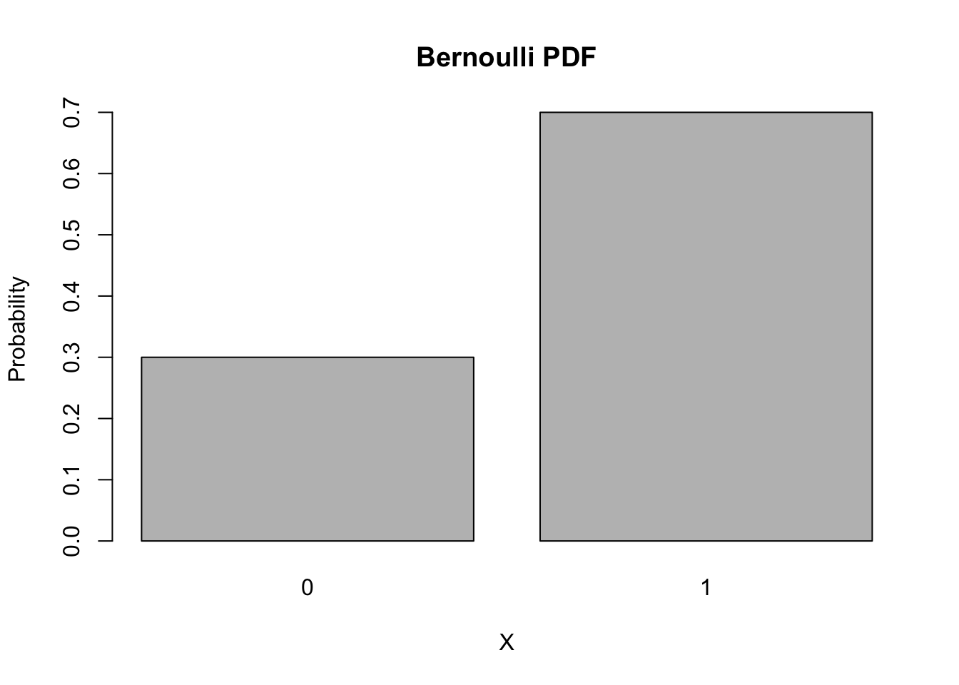
We will explore CDFs and inverse CDFs more in the following sections.
5.2.2 The Binomial Distribution
Notice we used the binom functions with size = 1 to explore the Bernoulli distribution. You may ask, “What if we change the size argument?”. It turns out that this the same as asking, “What is the distribution of the sum of several Bernoulli variables?”
We call that distribution the binomial distribution. It is the same as counting the number of successes x in size attempts, with probability p of success per attempt. Sampling from a binomial distribution is simple,
rbinom(1, size = 20, p = 0.7)## [1] 14That is a single measurement from this distribution, but we can just as easily simulate many of them,
rbinom(15, size = 20, p = 0.7)## [1] 13 17 12 16 14 18 11 11 14 13 14 17 14 15 10We can plot the results if we simulate too many to examine directly,
dat <- rbinom(1000, size = 20, p = 0.7)
barplot(table(dat), ylab = "counts")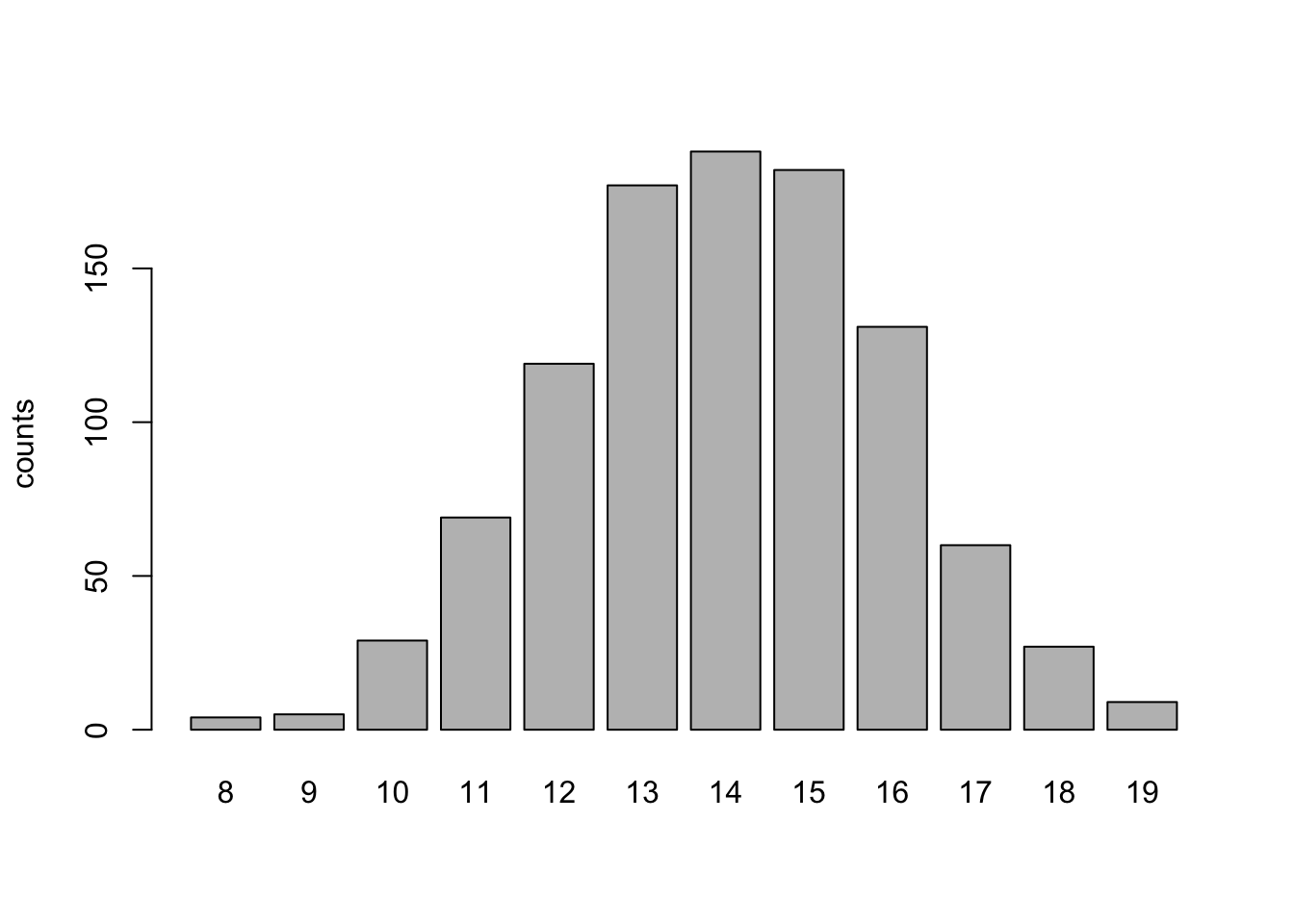
Distribution Functions
The probability density function (PDF) of the binomial distribution is given by: \[f(x|n,p) = \Pr(X = x) = {n\choose x}p^x(1-p)^{n-x}\]
The function that computes this automatically is dbinom(). The d stands for “density” and the binom stands for “binomial”. Suppose we want the probability of seeing 12 successes in 20 attempts, we can do this easily with,
dbinom(x = 12, size = 20, p = 0.7)## [1] 0.1143967In fact, we can easily obtain and draw the entire distribution,
barplot(height = dbinom(0:20, size = 20, p = 0.7), names.arg = 0:20,
        main = "Binomial PDF", xlab = 'X', ylab = 'Probability')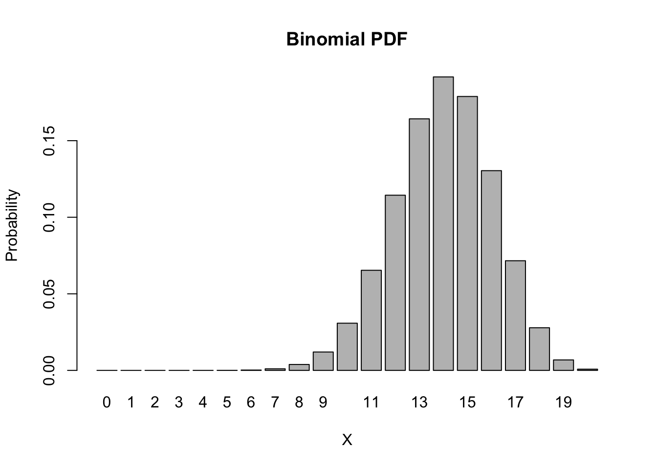
The cumulative distribution function (CDF) of the binomial distribution is given by: \[F(q|n,p) = \Pr(X \leq q) = \sum_{k=0}^q f(k|n,p)\]
Suppose we want the probability of seeing at most 12 successes in 20 attempts, we can do this easily with,
pbinom(q = 12, size = 20, p = 0.7)## [1] 0.2277282In fact, we can easily obtain and draw the entire CDF,
barplot(height = pbinom(0:20, size = 20, p = 0.7), names.arg = 0:20,
        main = "Binomial CDF", xlab = 'X', ylab = 'Probability')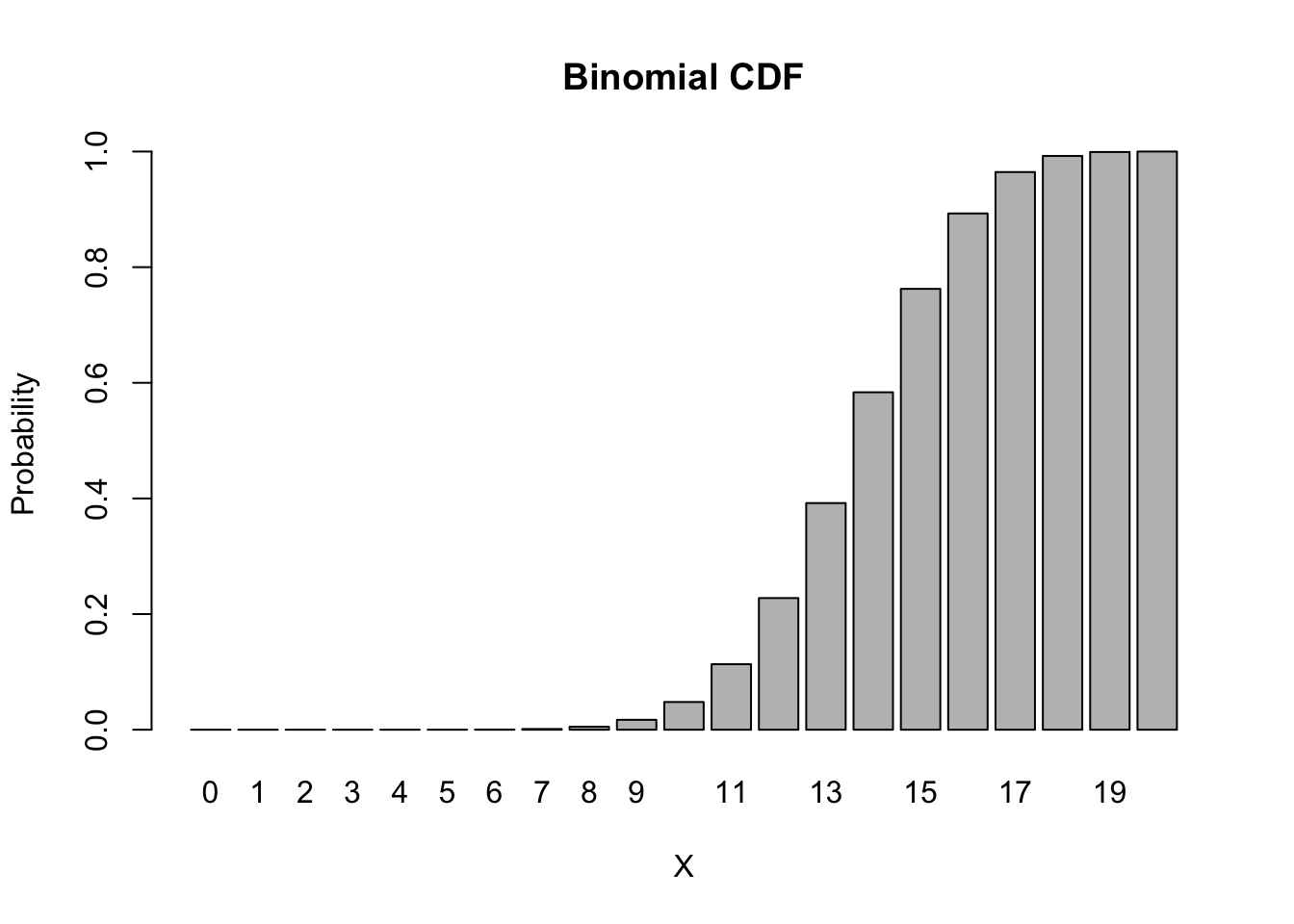
We illustrate the relationship between the PDF and the CDF in the following plot,
par(mfrow = c(1,2))
barplot(height = dbinom(0:20, size = 20, p = 0.7), names.arg = 0:20, ylim = c(0,1),
main = "Binomial PDF", xlab = 'X', ylab = 'Probability',
col = c(rep("blue", 15), rep("gray", 8)))
barplot(height = pbinom(0:20, size = 20, p = 0.7), names.arg = 0:20, ylim = c(0,1),
main = "Binomial CDF", xlab = 'X', ylab = 'Probability',
col = c(rep("gray", 14), "blue", rep("gray", 6)))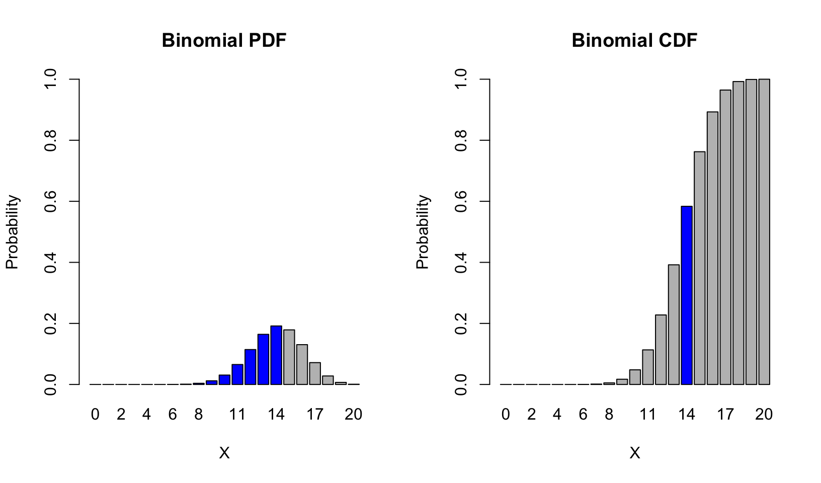 Notice that the value of the CDF at \(X = 14\) corresponds to the sum of the PDF from \(X = 0\) to \(X = 14\).
Properties of Distributions
Note that the sum of the distribution is,
sum(dbinom(0:20, size = 20, p = 0.7))## [1] 1And we can obtain the expectation,
sum(0:20 * dbinom(0:20, size = 20, p = 0.7))## [1] 14Which is exactly correct, knowing that \(\text{E}(X) = np = 20 \cdot 0.7\).
The variance is given by,
sum((0:20 - 20 * 0.7)^2 * dbinom(0:20, size = 20, p = 0.7))## [1] 4.2Which is equal to \(\text{Var}(X) = np(1-p) = 20 \times 0.7 \times 0.3\).
Exercises
Calculate the sum of 20 draws from a Bernoulli distribution with probability \(p\), and report the result.
Obtain a vector of 1000 draws from the Binomial(n = 20, p = 0.7) distribution and compute the sample mean and sample variance. Do they agree with our predictions?
5.2.3 The Poisson Distribution
The Poisson distribution is a discrete distribution which was designed to count the occurrences of something in a particular time interval. A common (approximate) example is counting the number of customers who enter a bank in a particular hour. The Poisson distribution often looks a lot like the binomial distribution, however, the number counted could, theoretically, be infinite which is one way to distinguish the two distributions. We traditionally call the expected number of occurrences \(\lambda\) or lambda.
As with the binomial, we can easily sample from the Poisson using the rpois() function,
rpois(n = 10, lambda = 14)## [1] 11 18 13 9 13 10 17 20 8 10We can also plot many samples from this lambda = 14 Poisson distribution,
data = rpois(n = 1000, lambda = 14)
barplot(table(data))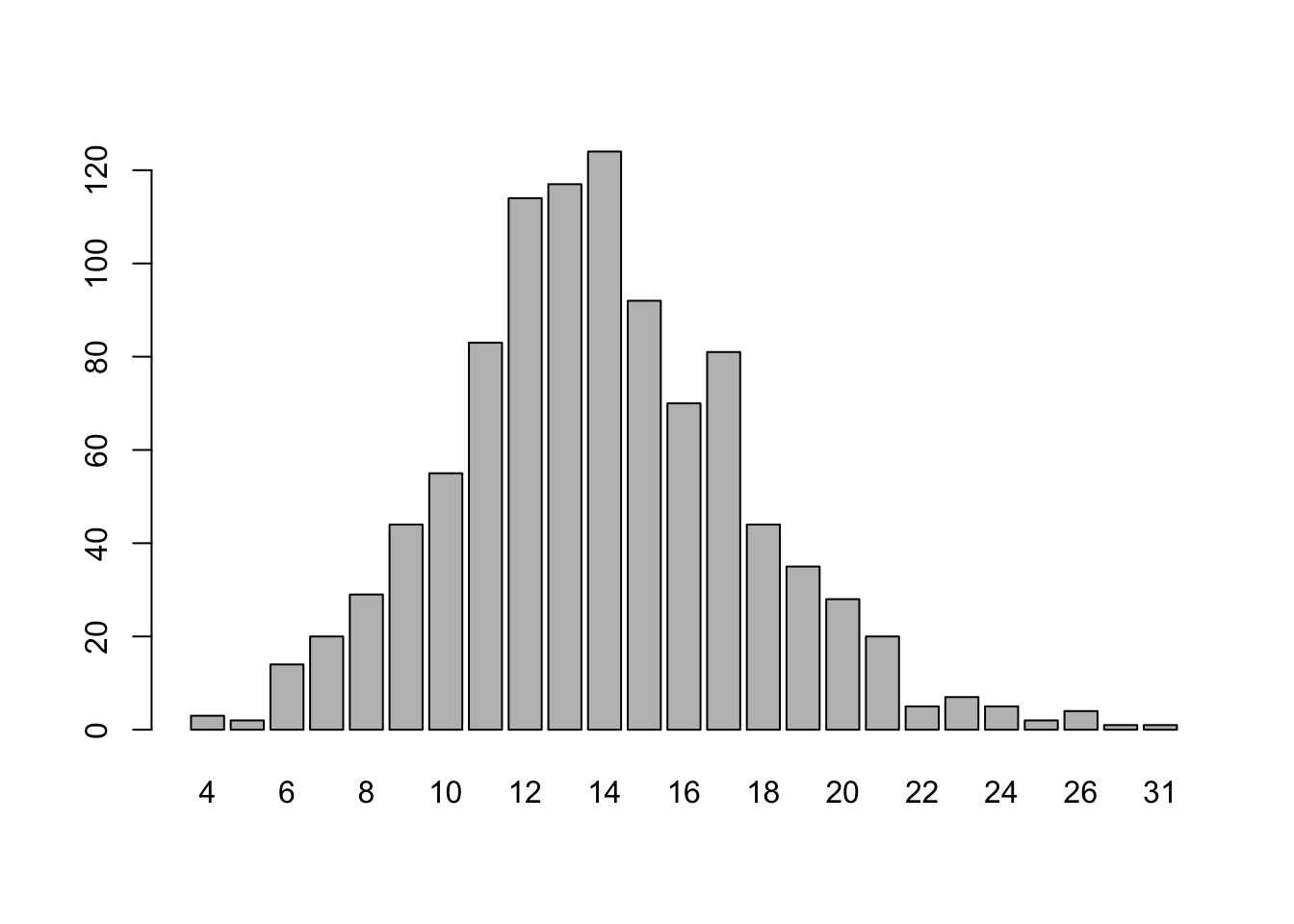
Distribution Functions
The probability density function (PDF) of the Poisson distribution is given by: \[f(x|\lambda) = \Pr(X = x) = \frac{\lambda^x e^{-x}}{x!}\] where \(e\) is equal to 2.7182818 and \(!\) is the factorial operator.
The function that computes this automatically is dpois(). The d stands for “density” and the pois stands for “Poisson”. Suppose we want the probability of seeing 12 occurrences, we can do this easily with,
dpois(x = 12, lambda = 14)## [1] 0.09841849In fact, we can easily obtain and draw the main part of the distribution,
barplot(height = dpois(0:30, lambda = 14), names.arg = 0:30,
        main = "Poisson PDF", xlab = 'X', ylab = 'Probability')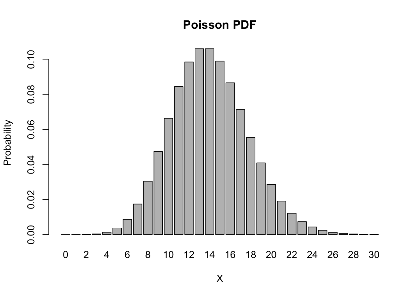
Note that this looks very much like the shape of the binomial distribution from the previous example. This is no coincidence, since the Binomial(20, 0.7) and the Poisson(14) distributions are closely related (note that \(20 \cdot 0.7 = 14\)).
The cumulative distribution function (CDF) of the binomial distribution is given by: \[F(q|\lambda) = \Pr(X \leq q) = \sum_{k=0}^q f(k|\lambda)\]
Suppose we want the probability of seeing at most 12 occurrences, we can do this easily with,
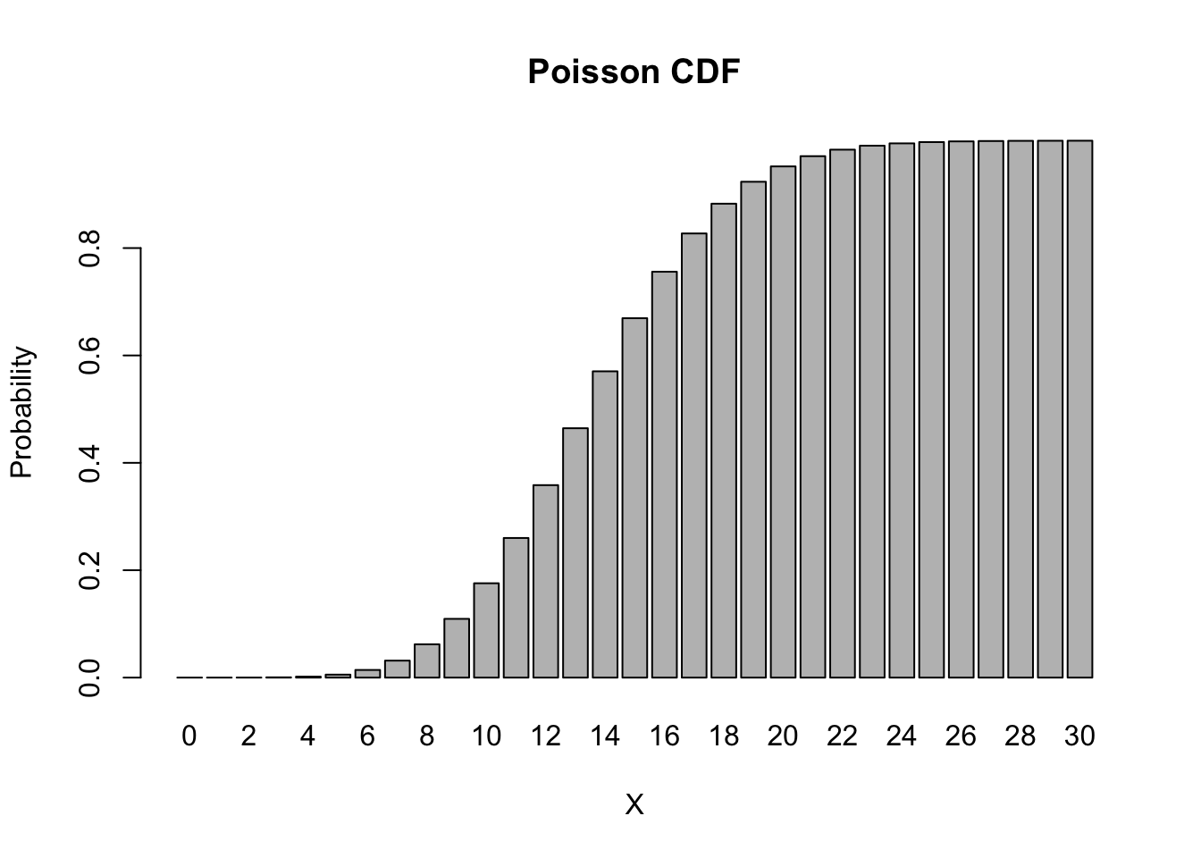
ppois(q = 12, lambda = 14)## [1] 0.3584584In fact, we can easily obtain and draw the main part of the CDF,
barplot(height = ppois(0:30, lambda = 14), names.arg = 0:30,
        main = "Poisson CDF", xlab = 'X', ylab = 'Probability')