3.2 Bivariate Numerical Summaries

3.2.1 Covariance

Previously, we used the var() function to calculate the variance statistic of a sample for a single variable. A closely related statistic is the covariance, calculated by the cov() function.

cov(weight, age)

## [1] 26.63442

The covariance will be positive if the two variables tend to have large/positive at the same time, and small/negative values at the same time. Unfortunately, we often cannot tell what is a “large” value of the covariance without some additional information, most often how much the two variables vary individually. We will explore how to handle that in the next statistic.

Below, we break down the covariance into the contributions by each point. Notice that the points in the first and third quadrants have positive contributions, while the points in the second and fourth quadrants have negative contributions. Also note that the points farthest in the corners, far from the mean of both variables or the centroid, have the biggest contributions. (Don’t worry about the large block of code, we will not expect you to plot things like this, but it is an illustration of what R is capable of.)

covparts <- (age - mean(age)) * (weight - mean(weight))
plot(age, weight, 
     main = "Scatterplot with point size=covariance contribution",
     col = ifelse(covparts > 0, rgb(0, 0, 1, 0.6), rgb(1, 0, 0, 0.6)),
     pch = 16, cex = abs(covparts)^0.33, 
     xlab = "Age", ylab = "Weight")
abline(h = mean(weight), col = "black")
abline(v = mean(age), col = "black")
legend("bottomright", legend = c("Positive", "Negative"),
       pch = 16, col = c(rgb(0,0,1,0.6), rgb(1,0,0,0.6)))
labs <- c(4,16,18,22)
text(age[labs], weight[labs], 
     round(covparts[labs], 1), adj = c(0.5, 0.25),
     cex = abs(covparts[labs])^0.1 / 1.5)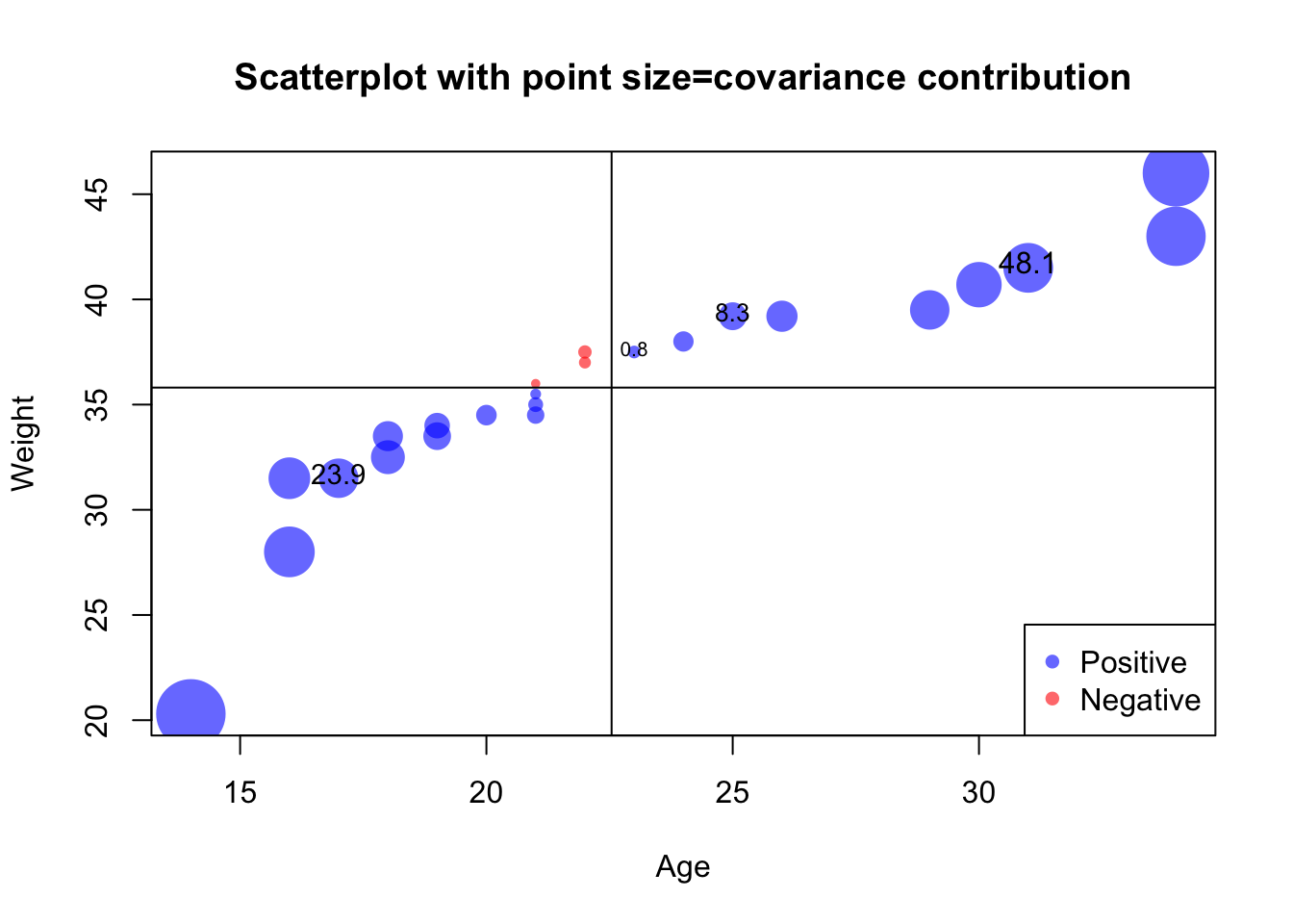

3.2.2 Correlation

We can calculate the sample correlation using the cor() function.

cor(weight, age)

## [1] 0.908391

Correlation solves one of the problems with the covariance by scaling by the standard deviations of the two variables.

cov(weight, age) / (sd(weight) * sd(age))

## [1] 0.908391

The correlation will always be between -1 and 1, with 1 representing perfect linearity sloping upward, and -1 representing perfect linearity sloping downward.