Introduction to Statistics with R

5.4 Limit Theorems

5.4.1 The Law of Large Numbers

We can make a plot of the propotions of 500 coin flips with code like the following. Note the use of the cumsum() function, which calculates a cumulative sum that adds up the flips that are “H”. In the long run, we get “H” about half the time.

set.seed(1234)
flips <- sample(c("heads", "tails"), size = 500, replace = TRUE)
plot(cumsum(flips == "heads") / (1:length(flips)), type = "l", ylim = c(0,1),  
     main = "Coin Flips", xlab = "Number of flips", ylab = "Proportion of heads")
abline(h = 0.5, col = "red")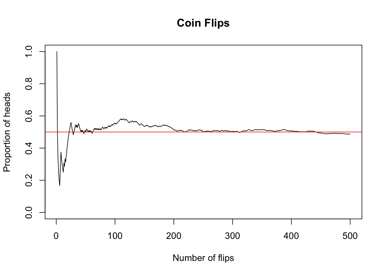

The theorem that guarantees this is called the Law of Large Numbers (LLN), a fundamental result proven by mathematician Jacob Bernoulli in 1713. The LLN ensures that casinos make money in the long run, among other important results, by guaranteeing that random variables tend to turn out the way we expect them to, at least in the long run.

Discussion

What does the Law of Large Numbers say about randomizing experiment subjects into treatment and control groups?

5.4.2 The Central Limit Theorem

Suppose we revisit the Uniform distribution from Section 5.3.2. Let’s take three samples of different sizes, namely 10, 20 and 50.

set.seed(1727498)
u10 <- runif(n = 10, min = -1, max = 2)
u20 <- runif(n = 20, min = -1, max = 2)
u50 <- runif(n = 50, min = -1, max = 2)

If we examine the samples, we can, more or less, see the Uniform distribution in all three cases.

par(mfrow = c(1, 3))
hist(u10, xlim = c(-2, 3), xlab = "x", main = "Histogram of 10 uniform samples")
hist(u20, xlim = c(-2, 3), xlab = "x", main = "Histogram of 20 uniform samples")
hist(u50, xlim = c(-2, 3), xlab = "x", main = "Histogram of 50 uniform samples")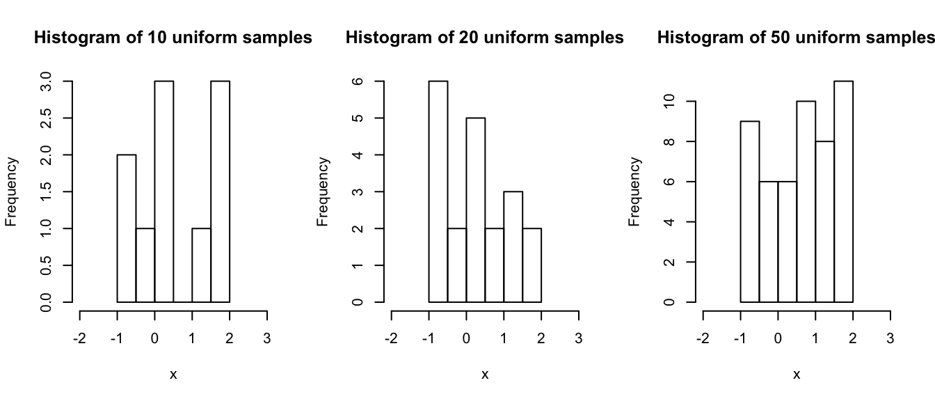

Now let’s look at how Normal these samples look. Note that all three plots have characteristic, obviously non-Normal tails on each end.

par(mfrow = c(1, 3))
qqnorm(u10, pch = 16, col = rgb(0, 0, 0, 0.5), main = "Q-Q Plot: 10 uniform samples")
qqline(u10, col = rgb(1, 0, 0, 0.6))
qqnorm(u20, pch = 16, col = rgb(0, 0, 0, 0.5), main = "Q-Q Plot: 20 uniform samples")
qqline(u20, col = rgb(1, 0, 0, 0.6))
qqnorm(u50, pch = 16, col = rgb(0, 0, 0, 0.5), main = "Q-Q Plot: 50 uniform samples")
qqline(u50, col = rgb(1, 0, 0, 0.6))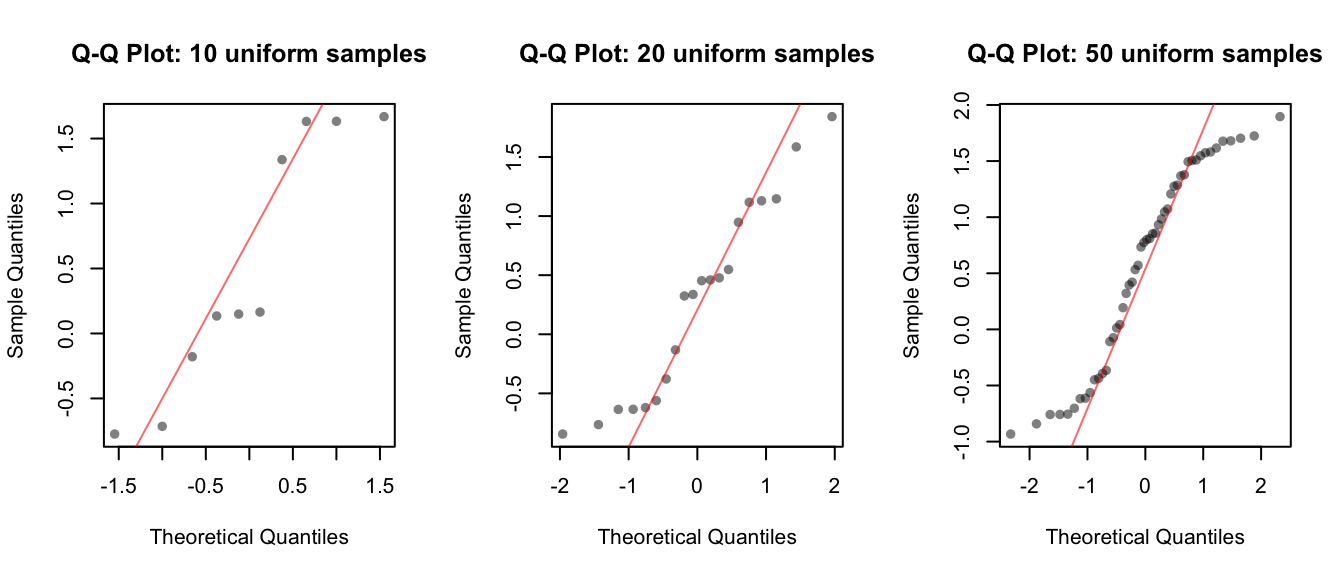

Now suppose we consider the sample means. We can calculate them simply enough,

c(mean(u10), mean(u20), mean(u50))

## [1] 0.5051040 0.2898156 0.5802317

Given the samples we took, these numbers are just constant numbers. However, if we were to take another sample, say of size 10, we would get a different number for the sample mean. Like so,

mean(runif(n = 10, min = -1, max = 2))

## [1] 0.8113241

Because this number is different every time we run it, this sample mean is a random variable too! It has a different distribution than the distribution of the samples themselves.

Let’s calculate this random sample mean many times. The replicate() function makes this very easy.

set.seed(81793)
u10bar <- replicate(1000, mean(runif(n = 10, min = -1, max = 2)))
u20bar <- replicate(1000, mean(runif(n = 20, min = -1, max = 2)))
u50bar <- replicate(1000, mean(runif(n = 50, min = -1, max = 2)))

If we look at the histograms of the sampling distributions, we see the Normal bell-curve appear more clearly with larger sample sizes.

par(mfrow = c(1, 3))
hist(u10bar, xlim = c(-2, 3), breaks = 10,
     xlab = "x", main = "1000 sample means of size 10")
hist(u20bar, xlim = c(-2, 3), breaks = 10,
     xlab = "x", main = "1000 sample means of size 20")
hist(u50bar, xlim = c(-2, 3), breaks = 10,
     xlab = "x", main = "1000 sample means of size 50")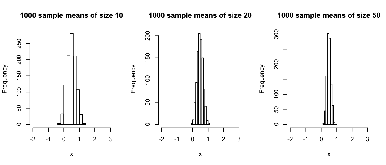

If we look at the Q-Q plots for our sampling distributions, we see that the sampling distribution is already close to Normal (we can tell because the points are close to the Q-Q line) even with samples of size 10. The normality becomes even stronger with sample sizes 20 and 50.

par(mfrow = c(1, 3))
qqnorm(u10bar, pch = 16, col = rgb(0, 0, 0, 0.5),
       main = "1000 sample means of size 10")
qqline(u10bar, col = rgb(1, 0, 0, 0.6))
qqnorm(u20bar, pch = 16, col = rgb(0, 0, 0, 0.5),
       main = "1000 sample means of size 20")
qqline(u20bar, col = rgb(1, 0, 0, 0.6))
qqnorm(u50bar, pch = 16, col = rgb(0, 0, 0, 0.5),
       main = "1000 sample means of size 50")
qqline(u50bar, col = rgb(1, 0, 0, 0.6))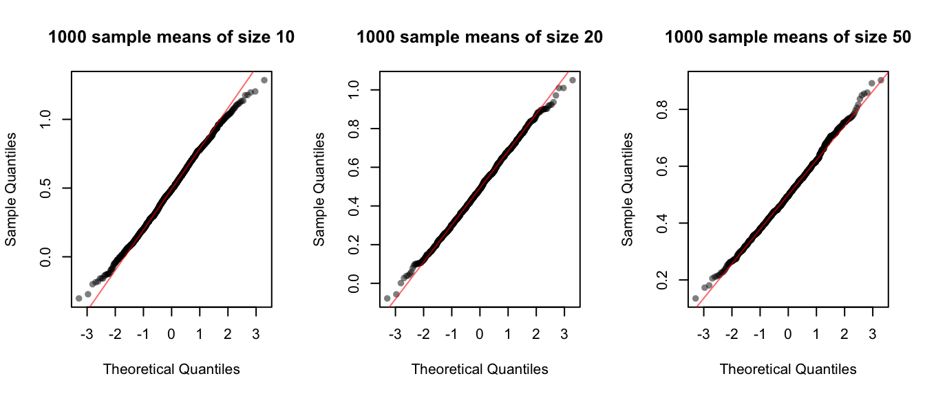

This is no coincidence! We have a powerful theorem that shows that this is practically guaranteed to happen for the Uniform and many more distributions. The Central Limit Theorem (CLT) states, roughly, that for most distributions that we care about, as we increase the sample size used to calculate the sample mean, the sampling distribution of the sample mean will become more and more Normal.