7.4 Confidence and Prediction Intervals

If you have a new data point (say DC), you can generate confidence and prediction intervals (based on the fitted model) for this point rather easily using the function predict():

First let’s look at the DC values:

print(DC)

## # A tibble: 1 × 5
##           State Y2016 Y2012 Y2008 Y2004
##           <chr> <dbl> <dbl> <dbl> <dbl>
## 1 Washington DC  0.91  0.91  0.92  0.89

Notice that the proportion of Democratic voters in the 2012 election for DC is far outside any of our other observed values (91%). We need to be particularly careful about making predictions based off this point because we would be extrapolating beyond the range of our data.

We can use the predict() function to get the confidence and prediction intervals for DC (for more info, use ?predict.lm)

The 95% confidence interval for DC, \(\mu_y\) | \(x =\) 0.91:

predict(lin.model, newdata = DC, 
        interval = "confidence", level = 0.95)

##        fit       lwr       upr
## 1 0.844835 0.8061764 0.8834937

The 95% prediction interval for DC, \(\widehat{y}_i\) | \(x =\) 0.91:

predict(lin.model, newdata = DC, 
        interval = "prediction", level = 0.95)

##        fit       lwr       upr
## 1 0.844835 0.7705959 0.9190742

7.4.0.1 Discussion

• Is DC inside the confidence interval?
• Is DC inside the prediction interval?

---

We can also plot the 95% confidence and prediction interval bands for the regression line.

# set up vector of equally spaced x values across the possible range
rangex <- data.frame(Y2012=seq(0, 1.0, by=0.05))

conf_interval <- predict(lin.model, newdata = rangex,
                         interval = "confidence", level = 0.95)
pred_interval <- predict(lin.model, newdata = rangex,
                         interval = "prediction", level = 0.95)

plot(Y2016 ~ Y2012, data = election, type="n",
     xlab = "2012 Election", ylab = "2016 Election", 
     main = "Proportion of Votes for Democratic Candidate By State")

DescTools::DrawBand(y = pred_interval[, 2:3],
                    x = rangex[,1], col = rgb(0.9, 0.9, 0.9, 0.5))
DescTools::DrawBand(y = conf_interval[, 2:3],
                    x = rangex[,1], col = rgb(0.8, 0.8, 0.8, 0.5))
points(Y2016 ~ Y2012, data = election,
       pch = 16, col = rgb(0, 0, 0, 0.5))
abline(lin.model, col = "red")

legend("topleft", legend=c("Prediction interval", "Confidence Interval"),
       pch=15, col=c("grey90", "grey80"))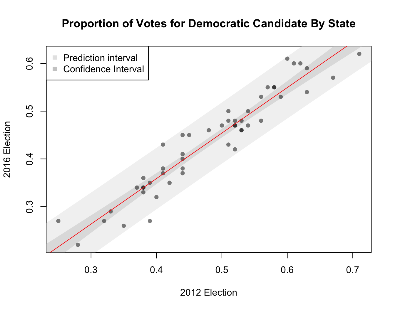

The confidence interval for (\(\widehat{y} | x\)) represents how the uncertainty in our estimate of the regression coefficient (the slope of the regression line) influences our prediction at specific values of \(x\).

The prediction interval is larger. This is because it accounts for both uncertainty of the regression line, and the the residual variation around the line.

Both intervals grow wider as the prediction point gets farther from the mean value of \(x\).