7.1 Linear Regression

Consider the simple linear model \[Y_i = \beta_0 + \beta_1 X_i\]
where \(Y_i\) and \(X_i\) are the proportion of democratic voters in 2016 and proportion of democratic voters in 2012 of the \(i^{th}\) state respectively, for \(i = 1, \ldots , 50\) (not including DC). \(\beta_0\) is the intercept, \(\beta_1\) is the slope. We might expect the proportion of Democratic voters in 2012 to be highly correlated to the proportion of Democratic voters in 2016.

lin.model <- lm(Y2016 ~ Y2012, data=election)
lin.model

## 
## Call:
## lm(formula = Y2016 ~ Y2012, data = election)
## 
## Coefficients:
## (Intercept)        Y2012  
##    -0.02235      0.95295

To see what output is stored in the object lin.model, use the names function:

names(lin.model)

##  [1] "coefficients"  "residuals"     "effects"       "rank"         
##  [5] "fitted.values" "assign"        "qr"            "df.residual"  
##  [9] "xlevels"       "call"          "terms"         "model"

You can extract these object elements, or pass them to other functions.

For example, the abline function will automatically pull the coefficients from the lin.model object and plot the corresponding line. The fitted.values in this object are our \(\hat{Y}_i\)’s, and we can plot them as well.

plot(Y2016 ~ Y2012, data = election,
     main = "Proportion of Votes for Democratic Candidate By State",
     xlab = "2012 Election", ylab = "2016 Election",
     pch = 16, col = rgb(0, 0, 0, 0.5))
abline(lin.model, col = "red")
points(lin.model$fitted.values ~ election$Y2012,
       pch = 17, col = rgb(0, 0, 1, 0.7))
legend("topleft", legend = c("Observed", "Fitted"),
       pch = c(16, 17), col = c(rgb(0, 0, 0, 0.5), rgb(0, 0, 1, 0.7)))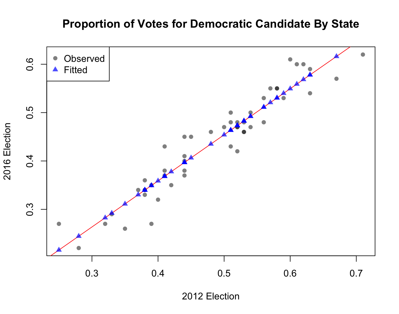

Discussion

• What observations are you able to draw from the plot?
• What assumptions do we need for linear regression? Do you think they are satisfied here?
• Are there any outliers?
• Are there any influential points?

---

The summary() function is a very useful function in R for many different classes of objects. Applying summary() to lin.model returns the standard output needed to get a basic understanding of the regression results: estimates for the coefficients, the SE’s, and t-tests along with the p-values for assessing statistical significance. These test whether our coefficients are sigificantly different from 0. Another way of saying this is that they test \(H_0: \theta=0\) vs. \(H_a: \theta \ne 0\). Note this is a two-tailed test.

summary(lin.model)

## 
## Call:
## lm(formula = Y2016 ~ Y2012, data = election)
## 
## Residuals:
##       Min        1Q    Median        3Q       Max 
## -0.079300 -0.022713  0.000465  0.019404  0.061641 
## 
## Coefficients:
##             Estimate Std. Error t value Pr(>|t|)    
## (Intercept) -0.02235    0.02148  -1.041    0.303    
## Y2012        0.95295    0.04364  21.838   <2e-16 ***
## ---
## Signif. codes:  0 '***' 0.001 '**' 0.01 '*' 0.05 '.' 0.1 ' ' 1
## 
## Residual standard error: 0.03152 on 48 degrees of freedom
## Multiple R-squared:  0.9086, Adjusted R-squared:  0.9066 
## F-statistic: 476.9 on 1 and 48 DF,  p-value: < 2.2e-16