5.1 Basic Simulation

5.1.1 Flipping Coins

R has many functions for simulating random variables. Suppose we want to simulate a single fair coin toss (precisely defined, we want “heads” half of the time, and “tails” the other half of the time). We can use the sample() function to accomplish this, with the following code:

sample(c("heads", "tails"), size = 1, replace = TRUE)

## [1] "tails"

Now suppose we want to toss a fair coin multiple times? We can change one of the arguments to achieve this (as always, you can use ? or help() to check the documentation at any time).

sample(c("heads", "tails"), size = 5, replace = TRUE)

## [1] "tails" "tails" "tails" "heads" "heads"

What if we want an unfair coin? We can do that too–this code will flip a coin with a 90% chance of coming up heads:

sample(c("heads", "tails"), size = 1, replace = TRUE, prob = c(0.9, 0.1))

## [1] "heads"

5.1.2 Rolling Dice

Now consider a six-sided die (plural dice). If it is a fair die, each side (labeled 1 through 6, inclusive) will have equal probability (1/6) of coming up. We can simulate this with sample() too.

sample(1:6, size = 1, replace = TRUE)

## [1] 4

As above, we can also simulate rolling multiple dice. Here we roll three six-sided dice:

sample(1:6, size = 3, replace = TRUE)

## [1] 5 6 1

We can also roll unfair dice. Here 6 should come up very often:

sample(1:6, size = 12, replace = TRUE,
       prob = c(1/10, 1/10, 1/10, 1/10, 1/10, 5/10))

##  [1] 6 5 6 6 6 6 6 6 1 6 6 1

5.1.3 Random Seeds

It is important to note that R uses a pseudorandom number generator to generate all of its (pseudo)random results. This is important because that allows us to set a random seed so that all of our work is reproducible. It is also important in a grading context because you may need to set the same seed as your grader in order to get the same, correct results. We can use set.seed() to set the random seed, and we should always see the same results from code run after setting the seed.

set.seed(1)
sample(1:6, size = 3, replace = TRUE)

## [1] 2 3 4

sample(1:6, size = 3, replace = TRUE)

## [1] 6 2 6

set.seed(1)
sample(1:6, size = 3, replace = TRUE)

## [1] 2 3 4

sample(1:6, size = 3, replace = TRUE)

## [1] 6 2 6

5.1.4 Plotting Results

If we want to flip a lot of coins or roll a lot of dice, it quickly becomes impractical to go through all the results by hand. One of the best ways to explore lots of data is to plot it in some way.

Suppose we flipped a coin 20 times and want to see the results. We can use code from above and from previous tutorials to summarize the data.

data <- sample(c("heads", "tails"), size = 20, replace = TRUE)
barplot(table(data))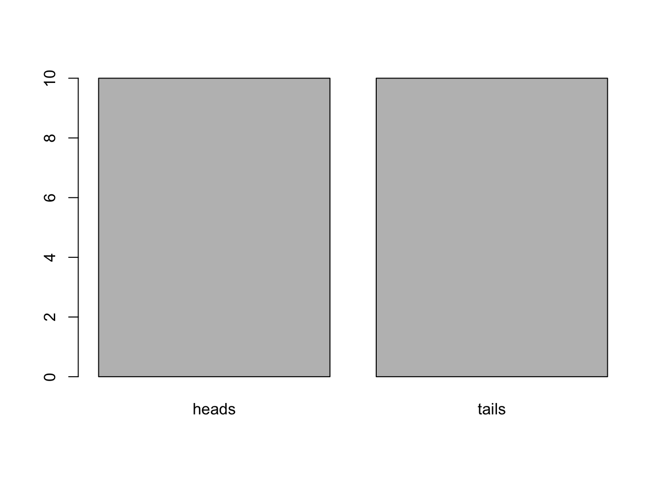

Now suppose we want to roll our unfair die 100 times.

data <- sample(1:6, size = 100, replace = TRUE,
               prob = c(1/10, 1/10, 1/10, 1/10, 1/10, 5/10))
barplot(table(data))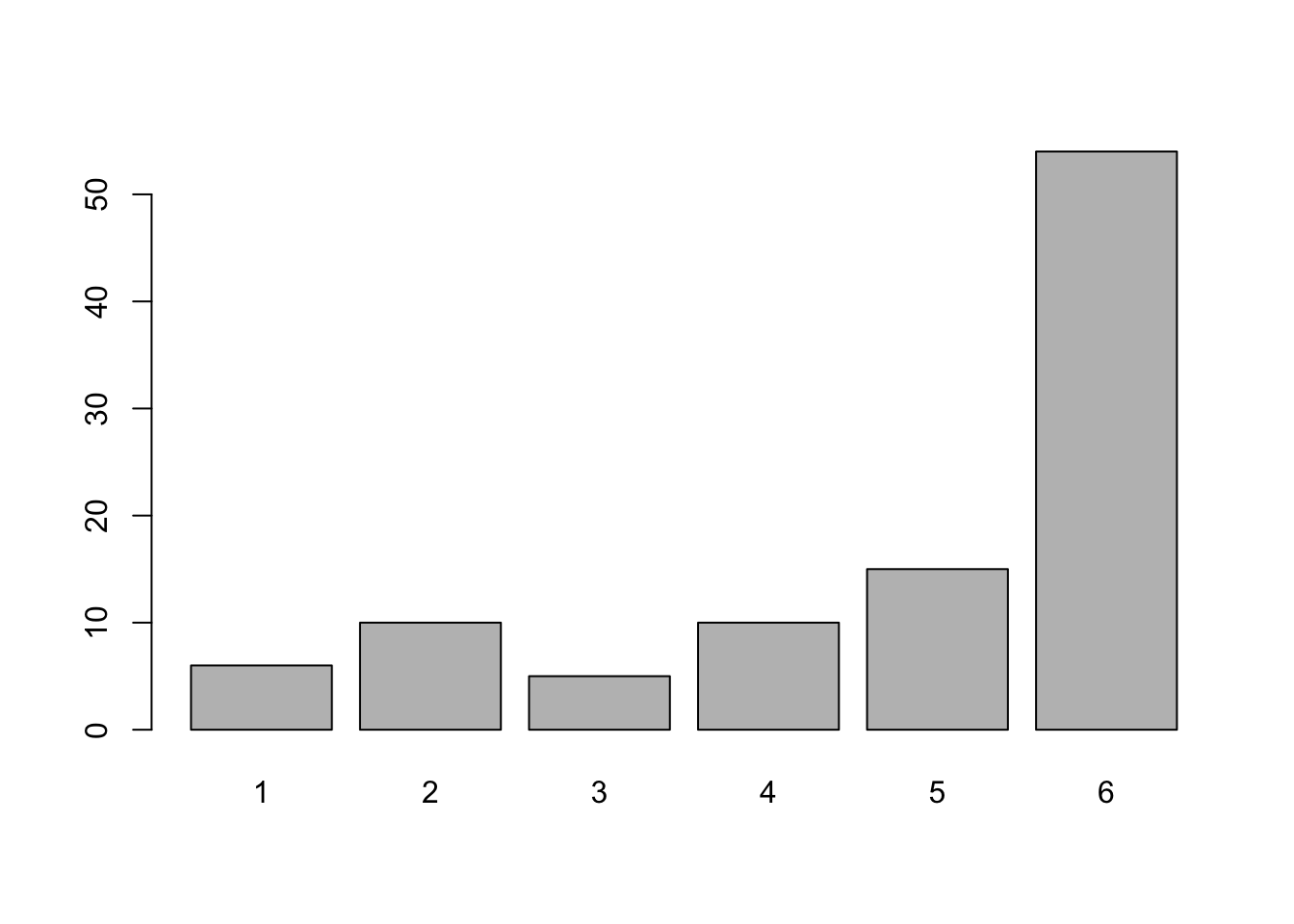

We can easily see which side is more likely to come up.